
Interpreting Piecewise Linear Functions 3
Loading the math board and drawing, please wait…
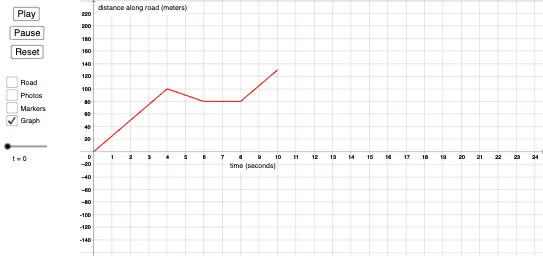
① This example demonstrates how to construct and dynamically interpret the graph of a piecewise linear function in GeoGebra, showing the connection of each linear segment and the change of slopes. ② Core mathematical concepts include piecewise functions, linear functions, properties of function graphs, and the idea of upper and lower Riemann sums. ③ Construction highlights: the Sequence command creates a parameter sequence, while the Segment command builds each line segment; key objects are the function graphs g_4, g_2, g_1, g_3, auxiliary points g_{y4}…g_{y1}, parameters t, a, b, c, d, t_1, list2, buttons button1‑button3, and geometric elements road_0, photo_{road}, left_{road}, right_{road}, mid_{road}. ④ Suitable for high‑school mathematics on functions and derivatives, as well as introductory university calculus for visualizing piecewise functions and integral approximations.
GeoGebra Commands & Parameters
Sequence((n, g(n)), n, 0, t_1) → list2Segment((-1.9, 0), (-1.1, 0)) → road_0Sequence(i - 0.4 < x < i + 0.4, i, 0, t_1) → photo_{road}Sequence(x = i - 0.4, i, 0, t_1) → left_{road}Sequence(x = i + 0.4, i, 0, t_1) → right_{road}Sequence(x = i, i, 0, t_1) → mid_{road}Sequence(Translate[car_p, Vector[(0, g(0)), (i - g_y(i), g(i))]], i, 0, t_1) → photo_rSegment((-1.9, 200), (-1.1, 200)) → road_{200}