
Interpreting Piece-wise Linear Functions by Mark Beckwith (2)
Loading the math board and drawing, please wait…
In collections
Algebra 1
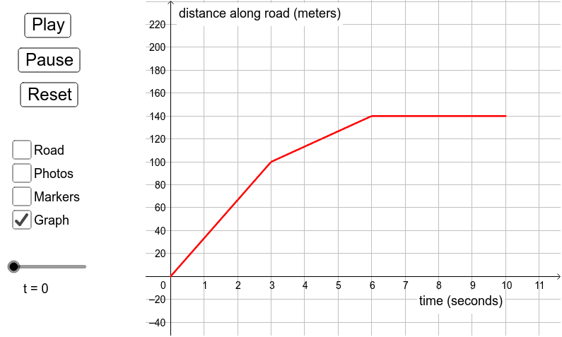
This example demonstrates the interpretation of piece-wise linear functions. Key mathematical concepts include piece-wise linear functions, linear functions, and linear regression. Using GeoGebra commands such as Sequence and Segment, the construction of piece-wise linear function graphs is illustrated. Suitable for high school mathematics education and learning.
GeoGebra Commands & Parameters
Sequence((n, g(n)), n, 0, t_1) → list2Segment((-1.9, 0), (-1.1, 0)) → road_0Sequence(i - 0.4 < x < i + 0.4, i, 0, t_1) → photo_{road}Sequence(x = i - 0.4, i, 0, t_1) → left_{road}Sequence(x = i + 0.4, i, 0, t_1) → right_{road}Sequence(x = i, i, 0, t_1) → mid_{road}Sequence(Translate[car_p, Vector[(0, g(0)), (i - g_y(i), g(i))]], i, 0, t_1) → photo_rSegment((-1.9, 200), (-1.1, 200)) → road_{200}
AI Drawing Prompt Reference
Draw a graph of a piecewise linear function to illustrate the linear relationships in different intervals. Start by drawing two horizontal reference lines, one at y=0 and another at y=200. Connect these lines with multiple line segments to form the image of the piecewise function. Place a moving car on each segment to visualize the changes in the function across different intervals. Finally, use dashed lines to indicate the range of each segment, helping to understand the piecewise definition of the function.
The prompt above was compiled from the original drawing commands and is for reference only.