Interactive Riemann Sums and Trapezoidal Approximation of Definite Integrals

GeoGebra Commands & Parameters

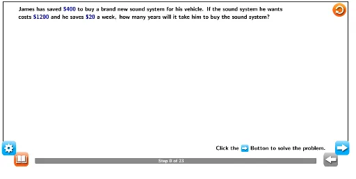
1. SelectedElement(S1) → s1
2. SelectedElement(T1) → t1
3. LaTeX((((("\text{James has saved \textcolor{#000099}{\textdollar{" * s1) * "}} to buy a brand new sound system for his vehicle. If the sound system he wants\\costs \textcolor{#000099}{\textdollar{") * t1) * "}} and he saves \textcolor{#000099}{\textdollar20} a week, how many years will it take him to buy the sound system?}")) → text1
4. LaTeX("\text{Read the problem carefully.}") → text2
5. LaTeX("\text{Reread the scenario and make a list of the known quantities.}") → text2_2
6. LaTeX("\text{Reread the problem again, identify the unknown quantity or variable. The scenario asks for the number of years.\\This is tricky because the quantity is given in terms of weeks. The variable to solve for first, then, is weeks.}") → text2_4
7. LaTeX((((("\text{The sound system costs \textcolor{#000099}{\textdollar{" * t1) * "}}. James has already saved \textcolor{#000099}{\textdollar{") * s1) * "}}. James will continue to save \textcolor{#000099}{\textdollar20} per week.}")) → text2_1
8. LaTeX("\text{Create an equation from the known quantities and variable(s).}") → text2_3
9. LaTeX((("\text{James’s goal is to save \textcolor{#000099}{\textdollar{" * t1) * "}}.}")) → text3
10. LaTeX((("\text{James has saved \textcolor{#000099}{\textdollar{" * s1) * "}} so far and has to save more to reach his goal.")) → text2_5
11. LaTeX("\text{Solve the equation for the variable.}") → text2_9
12. LaTeX((("\text{_______\textcolor{#000099}{ = {" * t1) * "}}}")) → text2_6
13. LaTeX((((("\text{\textcolor{#000099}{{" * s1) * "} + }______ \textcolor{#000099}{= {") * t1) * "}}}")) → text2_8
14. LaTeX((("\text{\textcolor{#000099}{−{" * s1) * "}}}")) → text2_{14}
15. LaTeX((("\text{\textcolor{#000099}{−{" * s1) * "}}}")) → text2_{11}
16. Segment(C, D) → f
17. LaTeX("\text{Interpret the solution in the context of the problem and convert to the appropriate units if necessary.}") → text2_{15}
18. LaTeX("\text{\textcolor{#000099}{\frac{1\;year}{52\;weeks}}}") → text2_{17}
19. LaTeX((("\text{\textcolor{#000099}{{" * week) * "} weeks \cdot \frac{1\;year}{52\;weeks}}}")) → text2_{20}
20. LaTeX((((("\text{\textcolor{#000099}{{" * week) * "} weeks \cdot \frac{1\;year}{52\;weeks}≈{") * sol) * "}\; years}}")) → text2_{19}
21. LaTeX("\text{James saved \textdollar}") → text5
22. LaTeX("\text{Sound system Costs \textdollar}") → text5_2
23. LaTeX((("\text{Step {" * Slider) * "} of 23}")) → text6
24. LaTeX((((("\text{\textcolor{#000099}{{" * s1) * "} + 20\mathit{x} = {") * t1) * "}}}")) → text2_{10}
25. LaTeX((((("\text{\textcolor{#000099}{{{" * s1) * "}+20\mathit{x}={") * t1) * "}}}")) → text2_{12}
26. LaTeX((("\text{\textcolor{#000099}{20\mathit{x}={" * sub) * "}}}")) → text2_{13}
27. LaTeX((("\text{\textcolor{#000099}{\frac{20\mathit{x}}{20}=\frac{{" * sub) * "}}{20}}}")) → text4
28. LaTeX((("\text{\textcolor{#000099}{\mathit{x}={" * week) * "}}}")) → text2_{16}
29. LaTeX("\text{James is saving \textcolor{#000099}{\textdollar20} a week for some unknown number of weeks to reach his goal. Let \textcolor{#000099}{\mathit{x}} represent the number of weeks.}") → text2_7
30. LaTeX("\text{In the equation, \textcolor{#000099}{\mathit{x}} represents weeks. The problem statement asks for the number of years it will take James\\to save for the sound system, so convert weeks to years. There are \textcolor{#000099}{52} weeks in a year.}") → text2_{18}
31. Segment(E, F) → g
32. Segment(G, H) → h
33. LaTeX("\text{2}") → text7
34. LaTeX("\text{3}") → text8
35. LaTeX("\text{1}") → text9
36. LaTeX("\text{4}") → text10
37. LaTeX((("\text{James will need to save for approximately \textcolor{#000099}{{" * sol) * "}} years, a little more than quarters of the year,\\to pay for the new sound system.}")) → text2_{22}
38. LaTeX("\text{The amount or number of a material or abstract thing not\\usually estimated by spatial measurement.}") → text12_3
39. LaTeX("\text{Each of four equal or corresponding parts into which something\\is or can be divided.}") → text12
40. LaTeX("\text{\textbf{Quantity:}}") → text12_1
41. LaTeX("\text{\textbf{Quarter:}}") → text12_2
42. Polygon(L, M, N, O) → poly1, l, m, n, o_1
43. LaTeX("\text{“}") → text14
44. LaTeX("\text{“}") → text14_2
45. LaTeX("\text{Click the Button to solve the problem.}") → text11
46. LaTeX("\text{\mathbf{Note:}“Use the (Data Kit) \\to return to the original problem \\or randomly generate a similar \\practice problem.\;\;and\;“Use \\the (Definition) to review\\words to know.}") → text13