
Interactive Demo of Linear Functions and Probability Distributions
Loading the math board and drawing, please wait…
In collections
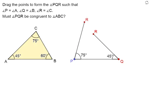
Exploring the Conditions for Congruence of 2 Triangles
Exploring Congruence of Triangles
This example demonstrates the geometric relationship between linear functions and Poisson/Binomial distributions through interactive graphics. Key math concepts include linear functions, Poisson distribution, binomial distribution, rational numbers, and perimeter. GeoGebra commands/objects used in construction are Vector, Point, Intersect, Segment, Sequence, DynamicCoordinates, Polygon, If, and Angle. Suitable for high school and above students to visualize function and probability distribution graphs and understand parameter effects.
GeoGebra Commands & Parameters
Vector(A, C1) → uPoint(Ray[A + (1, 0), A + (2, 0)]) → BVector(B, C2) → vIntersect(Ray[D, Rotate[D + (1, 0), 45°, D]], Ray[E, Rotate[E - (1, 0), (-(60°)), E]]) → FSegment(F, D) → kSequence((x(A) + (Length[u] * cos(t°)), y(A) + (Length[u] * sin(t°))), t, 0, 355, 5) → VPointsSegment(E, F) → jDynamicCoordinates(C1, x(ClosestPoint[VPoints, C1]), y(ClosestPoint[VPoints, C1])) → CSegment(A, C) → fSegment(A, B) → gSequence((x(B) + (Length[v] * cos(t°)), y(B) + (Length[v] * sin(t°))), t, 0, 355, 5) → UPointsDynamicCoordinates(C2, x(ClosestPoint[UPoints, C2]), y(ClosestPoint[UPoints, C2])) → C'Segment(C', B) → hIntersect(Ray[A, C], Ray[B, C']) → GPolygon({A, B, G}) → t1If(C ≟ G ∧ C' ≟ G, true, false) → closed1Segment(D, E) → iPolygon(D, E, F) → t3, l, m, nAngle(E, D, F) → αAngle(F, E, D) → βAngle(D, F, E) → γAngle(B, A, C) → δAngle(C', B, A) → εAngle(A, C, B) → ζ
AI Drawing Prompt Reference
Create an interactive graphic showing the geometric relationship between linear functions and Poisson/Binomial distributions. Include two vectors and an intersection point, generating rays from the vectors, and connecting the intersection to form a triangle. Display the trajectories of the vector endpoints with dynamic coordinates and draw line segments connecting these points. Finally, combine the triangle with the line segments to illustrate the relationship between functions and distributions, labeling key angles.
The prompt above was compiled from the original drawing commands and is for reference only.