
Integration Approximation: Upper Sum, Lower Sum & Trapezoids
Loading the math board and drawing, please wait…
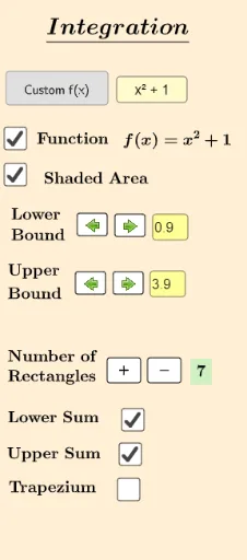
This GeoGebra example dynamically visualizes three classical methods for approximating definite integrals: the upper sum, lower sum, and trapezoidal sum. It demonstrates how rectangles and trapezoids under a function curve approximate the area when the interval is divided into n subintervals, and compares the accuracy as n increases. The core mathematical concepts include Riemann sums, the geometric meaning of definite integrals, convergence, and numerical integration fundamentals. The construction uses GeoGebra commands such as Integral, UpperSum, LowerSum, TrapezoidalSum, Sequence, If, Sum, Intersect, and Segment, with a slider n controlling the number of subdivisionscars, and text fields for bounds a and b. It is suitable for senior high school or introductory college calculus students to grasp approximation principles and compare numerical methods interactively, and serves as a powerful classroom demonstration tool.
GeoGebra Commands & Parameters
Integral(f, a, b) → cRectangleSum(f, a, b, n, 2) → eLowerSum(f, a, b, n) → gUpperSum(f, a, b, n) → dTrapezoidalSum(f, a, b, n) → jTextfield(a) → InputBox1Textfield(b) → InputBox2Sequence(a + (w * (b - a) / n), w, 0, n) → xvaluesSequence(f(a + (w * (b - a) / n)), w, 0, n) → yvaluesIf(n ≥ 1, B1 + "", "") → B6If(n ≥ 1, C1 + "", "") → C6If(n ≥ 2, D1 + "", "") → D6If(n ≥ 3, E1 + "", "") → E6If(n ≥ 4, F1 + "", "") → F6If(n ≥ 5, G1 + "", "") → G6If(n ≥ 6, H1 + "", "") → H6If(n ≥ 7, I1 + "", "") → I6If(n ≥ 8, J1 + "", "") → J6If(n ≥ 1, C2 + "", "") → C7If(n ≥ 2, D2 + "", "") → D7If(n ≥ 3, E2 + "", "") → E7If(n ≥ 4, F2 + "", "") → F7If(n ≥ 5, G2 + "", "") → G7If(n ≥ 6, H2 + "", "") → H7If(n ≥ 7, I2 + "", "") → I7If(n ≥ 8, J2 + "", "") → J7If(n ≥ 1, B2 + "", "") → If(n ≥ 10, L1 + "", "")If(n ≥ 1, B2 + "", "") → B7Sum(yvalues, n) → tIf(n ≥ 1, B9, If[n ≥ 2, B9 + C9]) → text15If(n ≥ 8, L1 + "", "") → L6If(n ≥ 8, M1 + "", "") → M6If(n ≥ 8, N1 + "", "") → N6If(n ≥ 8, O1 + "", "") → O6If(n ≥ 8, P1 + "", "") → P6If(n ≥ 8, Q1 + "", "") → Q6If(n ≥ 8, R1 + "", "") → R6If(n ≥ 8, S1 + "", "") → S6If(n ≥ 8, T1 + "", "") → T6If(n ≥ 8, U1 + "", "") → U6If(n ≥ 8, V1 + "", "") → V6If(n ≥ 8, K2 + "", "") → K7If(n ≥ 8, L2 + "", "") → L7If(n ≥ 8, M2 + "", "") → M7If(n ≥ 8, N2 + "", "") → N7If(n ≥ 8, O2 + "", "") → O7If(n ≥ 8, P2 + "", "") → P7If(n ≥ 8, Q2 + "", "") → Q7If(n ≥ 8, R2 + "", "") → R7If(n ≥ 8, S2 + "", "") → S7If(n ≥ 8, T2 + "", "") → T7If(n ≥ 8, U2 + "", "") → U7If(n ≥ 8, V2 + "", "") → V7If(n ≥ 9, K1 + "", "") → K6If(n ≥ 1, (Element[xvalues, 1], 0)) → x_1If(n ≥ 1, (Element[xvalues, 2], 0)) → x_2If(n ≥ 1, (Element[xvalues, 3], 0)) → x_3If(n ≥ 1, (Element[xvalues, 4], 0)) → x_4If(n ≥ 1, (Element[xvalues, 5], 0)) → x_5If(n ≥ 1, (Element[xvalues, 6], 0)) → x_6If(n ≥ 1, (Element[xvalues, 7], 0)) → x_7If(n ≥ 1, (Element[xvalues, 8], 0)) → x_8If(n ≥ 1, (Element[xvalues, 9], 0)) → x_9If(n ≥ 1, (Element[xvalues, 10], 0)) → x_{10}If(n ≥ 1, (Element[xvalues, 11], 0)) → x_{11}If(n ≥ 1, (Element[xvalues, 12], 0)) → x_{12}If(n ≥ 1, (Element[xvalues, 13], 0)) → x_{13}If(n ≥ 1, (Element[xvalues, 14], 0)) → x_{14}If(n ≥ 1, (Element[xvalues, 15], 0)) → x_{15}If(n ≥ 1, (Element[xvalues, 16], 0)) → x_{16}If(n ≥ 1, (Element[xvalues, 17], 0)) → x_{17}If(n ≥ 1, (Element[xvalues, 18], 0)) → x_{18}If(n ≥ 1, (Element[xvalues, 19], 0)) → x_{19}If(n ≥ 1, (Element[xvalues, 20], 0)) → x_{20}If(n ≟ 20, (b, 0)) → x_{21}Textfield(f) → InputBox3Intersect(p, eq1) → AIntersect(p, eq2) → BSegment(x_1, A) → f_1Segment(If[n ≥ 1, (Element[xvalues, n + 1], 0)], B) → s
AI Drawing Prompt Reference
Draw a function curve with the area under it shaded, illustrating three numerical integration approximations: lower sum, upper sum, and trapezoidal sum. Use a slider to control the number of subintervals, and input boxes for the integration bounds. As the slider changes, dynamically show the corresponding rectangles or trapezoids with distinct colors, and display their total areas alongside the exact integral value for comparison. Include the function curve, partition points, filled approximation shapes, and numerical area values that converge as the subdivision count increases.
The prompt above was compiled from the original drawing commands and is for reference only.