Integral Examples from Function List with Numerical Summation

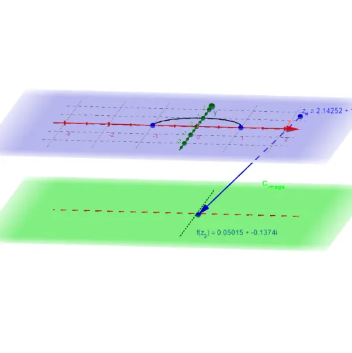
This GeoGebra example demonstrates how to select integrand functions from a predefined list and visualize their definite integrals as Cartesian curves, accompanied by numerical summation of integral terms. Core mathematical concepts include the geometric meaning of definite integrals, function list element selection, sequence summation and accumulation, parametric curve plotting, and vector/segment geometric construction. The construction relies on key GeoGebra commands: Integral for computing antiderivatives, Sequence and Zip for iterating over the fnlist function collection, SelectedElement and Element for picking specific functions such as f_{(z#)}, CurveCartesian for drawing parametric curves, Vector and Segment for geometric annotations, Textfield for dynamic labels, and ESum for displaying the accumulated sum; additional objects like Sphere, Intersect, C_{domain}, and C_{image} suggest domain-boundary or spatial intersection handling. Suitable for high school calculus electives and introductory university mathematical analysis, this resource supports classroom demonstrations of integral-list interactions and independent student exploration of function integral behavior.