Inference with Linear Regression (Work in Progress)

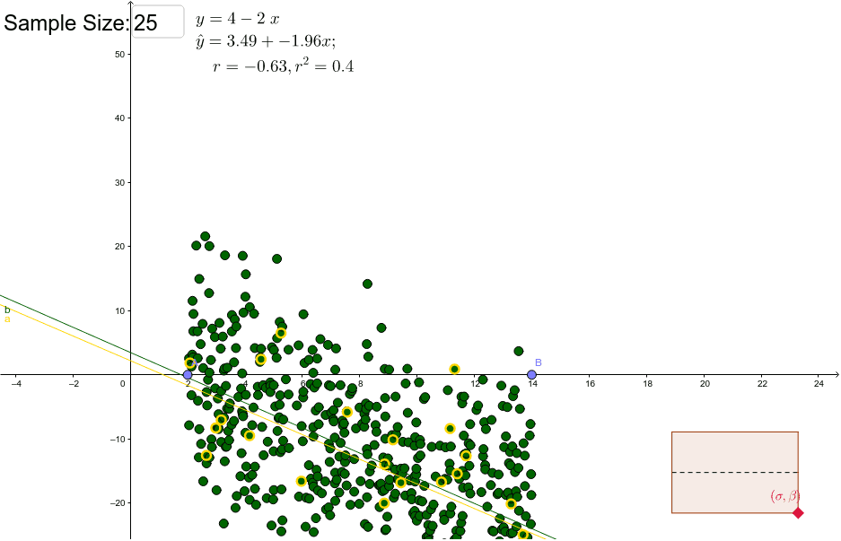
① This example demonstrates an interactive visualization for statistical inference in linear regression, including scatter plots, fitted lines, and confidence intervals. ② Core mathematical concepts include linear regression, least squares, Pearson's correlation coefficient (PMCC), standard deviations, sampling distribution of slope, and confidence intervals in inferential statistics. ③ Construction highlights: using GeoGebra commands such as Segment, Point, Polygon, FitLineY, SDY, SDX, PMCC, along with text fields and sliders, to dynamically adjust data points and observe changes in the regression line and computed statistics. ④ Suitable for high school or college statistics courses, it serves as a tool for teachers to demonstrate and students to explore the inference process in linear regression.