
Graphing Linear Inequalities by Andrew Knauft
Loading the math board and drawing, please wait…
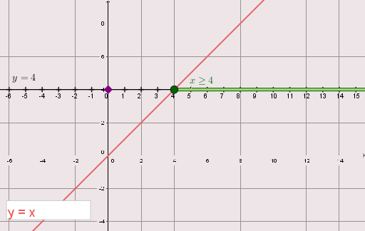
This example demonstrates how to graph the solution set of linear inequalities in a coordinate system. Key math concepts include linear inequalities, boundary lines, and solution regions. It utilizes GeoGebra commands such as Line, Sequence, Point, Intersect, DynamicCoordinates, Ray, and Textfield to construct the graph. Suitable for high school students learning to represent linear inequalities visually.
GeoGebra Commands & Parameters
Line(A, xAxis) → fSequence((n, handle), n, -10, 20) → list2Sequence(Text[n, (n - 0.2, handle - 0.55)], n, -10, 20) → list1Point(f) → BIntersect(f, h) → CDynamicCoordinates(B, If[abs(x(B) - x(C)) < ε, x(C), x(B)], handle) → DRay(D, D + (1, 0)) → gRay(D, D + (1, 0)) → iTextfield(h) → InputBox1
AI Drawing Prompt Reference
Draw the solution set of linear inequalities in a coordinate system by first plotting the x-axis, then generating a sequence of points from -10 to 20 and labeling their x-coordinates. Next, draw a line through the x-axis point and one of the sequence points, and find the intersection point with another line. From this intersection point, draw two rays along the positive x-axis, and label the x-coordinate at the intersection. Finally, add a text box in the coordinate system for inputting inequalities.
The prompt above was compiled from the original drawing commands and is for reference only.