
Indian Method for Square Root of Two
Loading the math board and drawing, please wait…
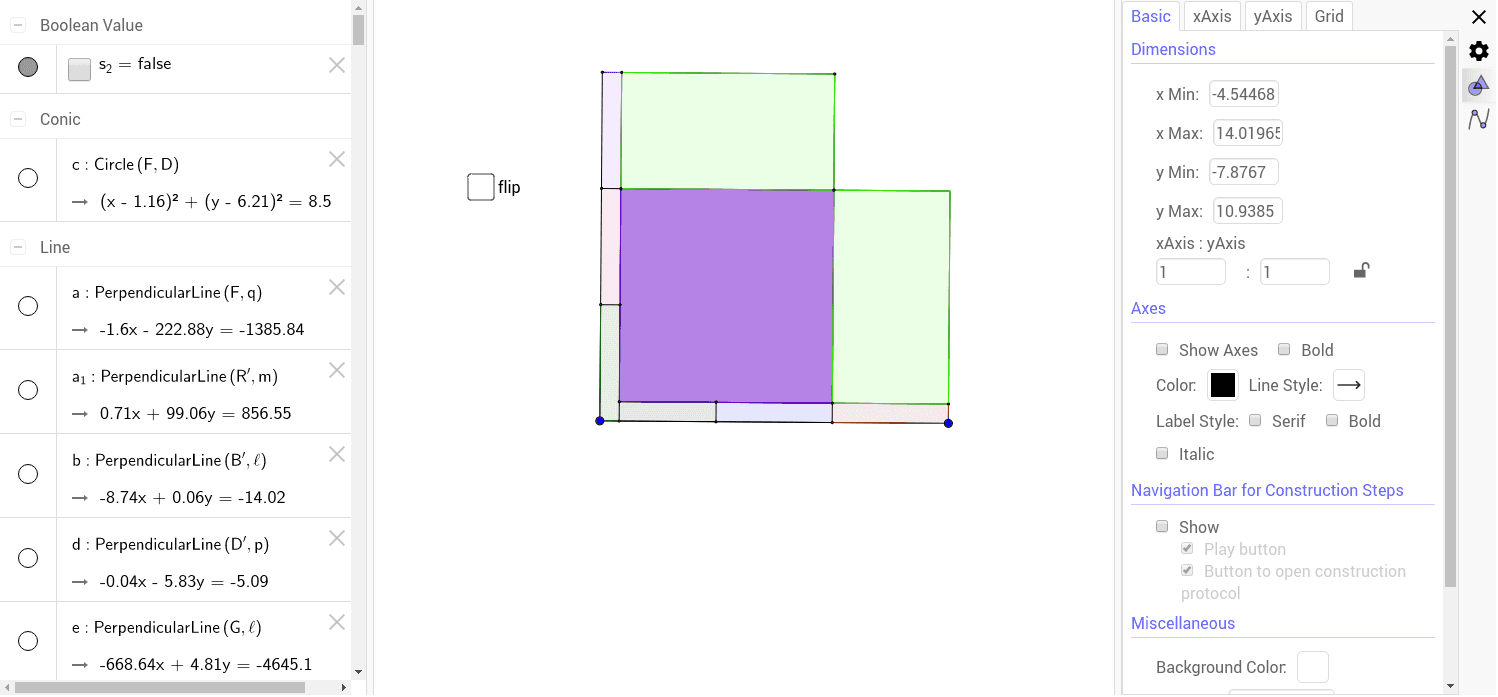
This example demonstrates an ancient Indian method for approximating the square root of two. It involves geometric constructions and properties of isosceles triangles. By constructing isosceles triangles and using geometric transformations, one can intuitively understand the approximation of the square root of two. Main commands used include Polygon, Dilate, OrthogonalLine, Intersect, Segment, Midpoint, Circle, Ray, Vector, Translate. Suitable for middle school and above students to learn geometric constructions and transformations.
GeoGebra Commands & Parameters
Polygon(A, B, 4) → poly1, f, g, h, i, C, DDilate(C, 2 / 3, D) → C'Dilate(C, 2 / 3, B) → C'_1OrthogonalLine(C', h) → jOrthogonalLine(C'_1, g) → kIntersect(j, k) → EIntersect(k, i) → FSegment(A, B) → lIntersect(l, j) → GSegment(C', E) → mSegment(E, C'_1) → nSegment(A, F) → pSegment(F, D) → qSegment(D, C') → rSegment(C'_1, B) → sMidpoint(r) → KOrthogonalLine(K, r) → g_1Intersect(g_1, l) → LDilate(B, 1 / 18, A) → B'Dilate(D, 1 / 18, A) → D'Circle(F, D) → cIntersect(c, p, 1) → HOrthogonalLine(H, p) → tOrthogonalLine(F, q) → aOrthogonalLine(B', l) → bOrthogonalLine(D', p) → dOrthogonalLine(G, l) → eIntersect(d, e) → IIntersect(g_1, d) → JIntersect(b, d) → MIntersect(t, b) → NIntersect(a, b) → OIntersect(r, b) → POrthogonalLine(D', p) → f_1Intersect(f_1, s) → QSegment(D', Q) → h_1Segment(F, O) → i_1Segment(H, N) → j_1Segment(M, Q) → k_1Segment(P, M) → l_1Segment(B', M) → m_1Segment(L, G) → n_1Segment(I, G) → p_1Segment(J, L) → q_1Ray(B, C'_1) → r_1Ray(D, C') → s_1Intersect(r_1, s_1) → RVector(J, L) → uVector(N, H) → vTranslate(R, u) → R'Translate(R, v) → R'_1Translate(R'_1, Vector[(0, 0)]) → STranslate(R'_1, Vector[(0, 0)]) → TTranslate(R'_1, Vector[(0, 0)]) → UOrthogonalLine(R'_1, r) → t_1OrthogonalLine(R', m) → a_1Intersect(t_1, a_1) → VSegment(C', R'_1) → b_1Segment(C'_1, R') → c_1Segment(R'_1, V) → d_1Segment(V, R') → e_1Dilate(R', 1 / 6, C'_1) → R''OrthogonalLine(R'', c_1) → f_2Intersect(f_2, m) → WIntersect(f_2, c_1) → ZVector(C'_1, R'') → wPolygon(E, W, R'', C'_1) → poly2, e_2, w_1, r'', c'_1Translate(E, w) → E'Translate(W, w) → W'Translate(R'', w) → R'''Translate(C'_1, w) → A_1Polygon(E', W', R''', A_1) → poly2', e', w', r''', a_2Translate(E', w) → E''Translate(W', w) → W''Translate(R''', w) → B_1Translate(A_1, w) → C_1Polygon(E'', W'', B_1, C_1) → poly2'', e'', w'', b_2, c_2Translate(E'', w) → E'''Translate(W'', w) → W'''Translate(B_1, w) → D_1Translate(C_1, w) → E_1Polygon(E''', W''', D_1, E_1) → poly2''', e''', w''', d_2, e_3Translate(E''', w) → F_1Translate(W''', w) → G_1Translate(D_1, w) → H_1Translate(E_1, w) → I_1Polygon(F_1, G_1, H_1, I_1) → poly3, f_3, g_2, h_2, i_2Translate(F_1, u_1) → J_1Translate(G_1, u_1) → K_1Translate(H_1, u_1) → L_1Translate(I_1, u_1) → M_1Polygon(J_1, K_1, L_1, M_1) → poly3', j_2, k_2, l_2, m_2Translate(J_1, w) → N_1Translate(K_1, w) → O_1Translate(L_1, w) → P_1Translate(M_1, w) → Q_1Polygon(N_1, O_1, P_1, Q_1) → poly3'', n_2, o_1, p_2, q_2Intersect(b_1, d_1) → R_1Polygon(O_1, V, R_1, C') → poly4, o_2, v_1, r_2, c'Polygon(D, P, O, F) → poly5, d_3, p_3, o, f_4Polygon(F, O, N, H) → poly6, f_5, o_3, n_3, h_3Polygon(H, N, B', A) → poly7, h_4, n_4, b', a_3Polygon(M, J, L, B') → poly8, m_3, j_3, l_3, b'_1Polygon(J, I, G, L) → poly9, j_4, i_3, g_3, l_4Polygon(I, Q, B, G) → poly10, i_4, q_3, b_3, g_4Segment(O, E) → t_2Segment(I, E) → k_3Polygon(M, O, E, I) → poly11, m_4, o_4, e_4, i_5Polygon(I, E, C'_1, Q) → poly12, i_6, e_5, c'_2, q_4Polygon(O, P, C', E) → poly13, o_5, p_4, c'_3, e_6