Illustrating Function Derivatives as Tangent-Line Slopes

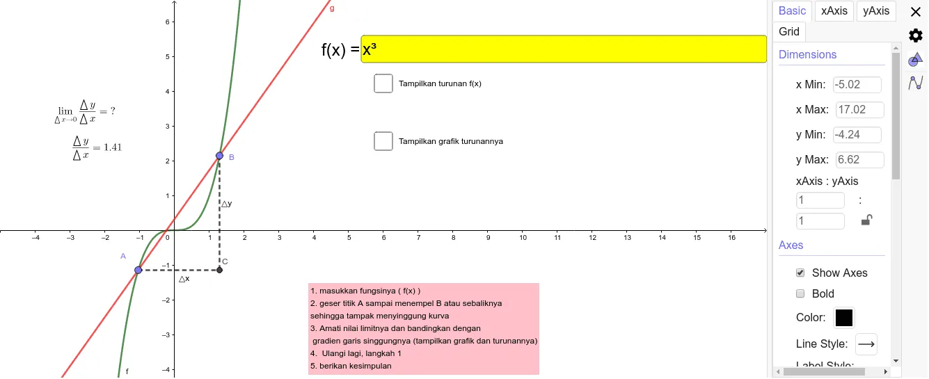
This example uses the tangent line to a function at a chosen point to visually demonstrate that the derivative equals the slope of the tangent line (local change rate). The key mathematics includes differentiation (Derivative), tangent construction (Tangent), slope (Slope), and the underlying idea of local behavior/limit (Limit) that motivates the derivative. In GeoGebra, the construction starts with Derivative to create the function’s derivative f', then places a point p on the graph, builds auxiliary lines with Line and OrthogonalLine, and uses Intersect to determine relevant intersection points. Tangent and Segment are used to display the tangent line and the important geometric segments, while Textfield annotates the computed slope/derivative value on the figure; InputBox1 and a limit-related workflow can be included to connect the numeric derivative with a limiting change-rate interpretation. It is designed for calculus instruction—especially for students learning derivatives visually via graphing and geometric reasoning.