
Hourly Temperature After Sunrise: Scatter Plot and Linear Modeling
Loading the math board and drawing, please wait…
In collections
CCSS IP Math I Unit 4 Lesson 2
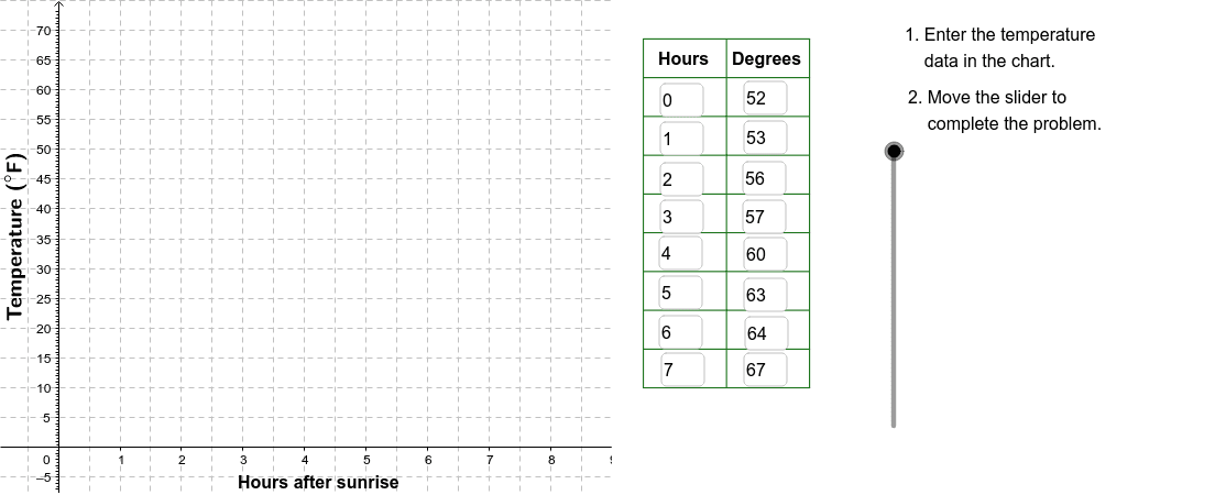
This example demonstrates a scatter plot of hourly temperature recorded after sunrise on a May morning, fitting linear and exponential functions to the data, and calculating the derivative of temperature change. In GeoGebra, the Corner command creates data points, Polygon draws the fitting shape, Textfield adds titles and labels, Sequence generates the time series, Line draws the linear regression, and VerticalText displays temperature values. It is suitable for high school or early university students learning coordinate geometry, function fitting, and differential analysis.
GeoGebra Commands & Parameters
Corner(2) → Corn2Corner(3) → Corn3Polygon(Corn1, Corn2, Corn3, Corn4) → poly1, corn1, corn2, corn3, corn4Textfield(A2) → InA2Textfield(A3) → InA3Textfield(A4) → InA4Textfield(A5) → InA5Textfield(A6) → InA6Textfield(A7) → InA7Textfield(A8) → InA8Textfield(A9) → InA9Textfield(B9) → InB9Textfield(B8) → InB8Textfield(B7) → InB7Textfield(B6) → InB6Textfield(B5) → InB5Textfield(B4) → InB4Textfield(B3) → InB3Textfield(B2) → InB2Sequence(Segment[(9.5, 10 + (6.5 * j)), (12.2, 10 + (6.5 * j))], j, 0, 9) → LnListSequence(Segment[(9.5 + (1.35 * j), 10), (9.5 + (1.35 * j), 68.5)], j, 0, 2) → LnList2Line(I, J) → FitLineVerticalText("\text{Temperature (}°\text{F)}") → DownLegend
AI Drawing Prompt Reference
Please draw a scatter plot of hourly temperature recorded after sunrise on a May morning, with linear and exponential function fitting. The graph should include data points, fitted curves, and the derivative of temperature change. Add titles and labels, generate the time series, draw the linear regression line, and display temperature values. Suitable for high school or early university students learning coordinate geometry, function fitting, and differential analysis.
The prompt above was compiled from the original drawing commands and is for reference only.