
Histogram Construction Examples
Loading the math board and drawing, please wait…
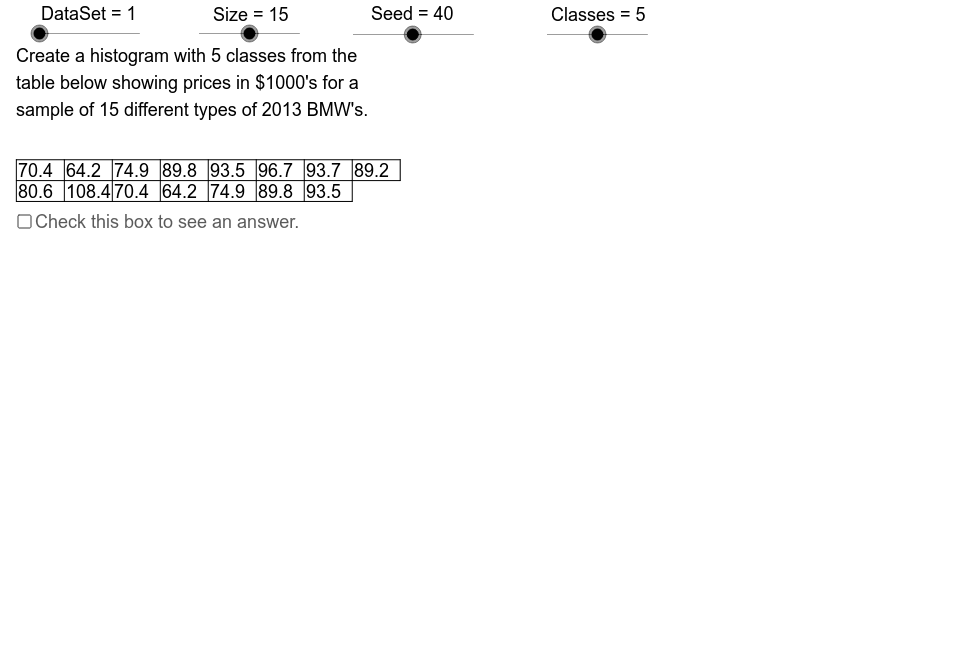
This example demonstrates how to construct histograms from data, visually representing data distribution. Key math concepts include data binning, frequency statistics, and bar chart creation. GeoGebra commands and objects used are Element, Sequence, Min, Max, If, KeepIf, Sort, CountIf, Append, Segment, Sum, VerticalText. Suitable for high school mathematics teaching, particularly for introductory probability & statistics and data processing practice.
GeoGebra Commands & Parameters
Element(AccSq, Data) → AccElement(RtSq, Mod[Seed, 8] + 1) → RateSequence(Mod[(Rate * k) + Start, 20] + 1, k, 0, 19, 1) → OptSqElement(DtSq, Data) → Dt0Sequence(Element[Dt0, Element[OptSq, k]], k, 1, Size) → SmpSqMin(SmpSq) → DtMnMax(SmpSq) → DtMxIf(C0 ≤ UB, C0, If[C1 ≤ UB, C1, If[C2 ≤ UB, C2, If[C3 ≤ UB, C3, C4]]]) → ClsWdSequence(DtMn + (k * ClsWd), k, 0, NoCls - 1) → LCLElement(LCL, 2) → LCL2If(C0 ≤ UB, 0, If[C1 ≤ UB, 0, If[C2 ≤ UB, 1, If[C3 ≤ UB, 2, 3]]]) → CWAccMax(Acc, CWAcc) → CnAccSequence(UCL1 + (ClsWd * k), k, 0, NoCls - 1) → UCLSequence(CountIf[Element[LCL, k] ≤ x ≤ Element[UCL, k], SmpSq], k, 1, NoCls) → FrqSqMax(FrqSq) → MxFrqSequence(TbTp - k, k, 0, 3) → TbLHSqElement(TbLHSq, 3) → TbLH2Element(TbLHSq, 1) → TbLH0Element(TbLHSq, 4) → TbLH3Element(TbLHSq, 2) → TbLH1Element(LCL, 1) → HAxMnElement(PlcSq, Data) → DPSequence(k, k, 1, 19) → StrtSqKeepIf(floor(20 / x) ≠ 20 / x, StrtSq) → RlPrmSqSequence(Element[SmpSq, k], k, 1, RwLn1) → DtRw1Sequence(Element[SmpSq, k], k, RwLn1 + 1, Size) → DtRw2Element(DDSq, Data) → DD0Sort(SmpSq) → SortSqCountIf(x > 0, RtSq) → RateNoElement(SclSq, Data) → ScaleElement(TSSq, Data) → TSSequence(If[k > 1, " + ", " "], k, 1, NoCls) → PlsSqSequence(" = ", k, 1, NoCls) → EqlSqSequence(DtMn + (k * ClsWd), k, 0, NoCls - 2) → LCLCn1Append(DtMn, LCLCn1) → LCLCn2Sequence(ClsWd, k, 1, NoCls - 1) → CWSq1Append(" ", CWSq1) → CWSq2Sequence(UCL1 + (ClsWd * k), k, 0, NoCls - 2) → UCLCn1Append(UCL1, UCLCn1) → UCLCn2Sequence("to", k, 1, NoCls) → ToSqSequence(If[Element[FrqSq, j] > 0, Sequence["|", k, 1, Element[FrqSq, j]], {" "}], j, 1, NoCls) → TlyElement(LCL, 1) → LCL1Segment(TbML, TbLR) → tbmdSegment(TbLL, TbMR) → tbbtSegment(TbUL, TbUR) → tbtpSum(FrqSq) → ChkSzCountIf(x ≠ (0, 0), Dt0) → DtCntSequence(Segment[(TbLf + (CllWd * k), TbLH0), (TbLf + (CllWd * k), TbLH2)], k, 0, RwLn2) → TbVLnIf(Mod[Size, 2] ≟ 1, Segment[TbLR, TbUR], Segment[TbMR, TbUR]) → tbrgSegment(GLL, GLR) → haxSegment(GUL, GLL) → vaxSequence(Segment[(GL - 0.3, VAdp(k)), (GL, VAdp(k))], k, 0, VAxMx) → VTcSequence(Segment[(HAdp(k), GB), (HAdp(k), VAdp(Max[Element[FrqSq, k], Element[FrqSq, k + 1]]))], k, 1, NoCls - 1) → BrSdSegment((GR, GB), (GR, VAdp(Element[FrqSq, NoCls]))) → rgsdSequence(Segment[(HAdp(k - 1), VAdp(Element[FrqSq, k])), (HAdp(k), VAdp(Element[FrqSq, k]))], k, 1, NoCls) → BrTpSequence(Text[DtMn + (k * ClsWd), (HAdp(k) - 0.3, GB - 0.9)], k, 0, NoCls) → HAxNmSqVerticalText("Frequency") → VAxTtlElement(TtlSq, Data) → TtlElement(HALSq, Data) → HALSequence(Text[k, (GL - 1.4, VAdp(k) - 0.3)], k, 0, VAxMx, VScl) → VAxNmSqSequence(Text[Element[LCL, k], (FDLf + 0.3, DLTp - (0.9 * k))], k, 1, NoCls) → LCLTxt2Sequence(Text[Element[FrqSq, k], (FDLf + 8.4, DLTp - (0.9 * k))], k, 1, NoCls) → FrqTxtSequence(Text[Element[DtRw2, k], (TbLf - 2.2 + (k * CllWd), TbLH2 + 0.15)], k, 1, RwLn2) → TxtRw2Sequence(Text[Element[DtRw1, k], (TbLf - 2.2 + (k * CllWd), TbLH1 + 0.15)], k, 1, RwLn1) → TxtRw1Sequence(Text[Element[UCL, k], (FDLf + 3.9, DLTp - (0.9 * k))], k, 1, NoCls) → UCLTxt2Sequence(Text[Element[ToSq, k], (FDLf + 2.8, DLTp - (0.9 * k))], k, 1, NoCls) → ToTxtSequence(Segment[(HAdp(k), GB), (HAdp(k), GB + 0.1)], k, 1, NoCls - 1) → HTc
AI Drawing Prompt Reference
Draw a histogram construction example. Start with a random sample dataset, compute its minimum and maximum, choose a suitable class width, and generate consecutive intervals with lower and upper bounds. Count frequencies in each interval and represent them as vertical bars whose heights match the counts. Also include a frequency distribution table with class ranges, frequency counts, and tally marks, framed by border lines. Show the overall data distribution and verify the total frequency.
The prompt above was compiled from the original drawing commands and is for reference only.