
Heat Equation Visualization Tool
Loading the math board and drawing, please wait…
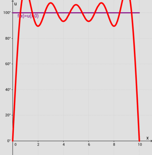
This example visualizes the heat equation. Key mathematical concepts include partial differential equations and heat conduction theory. Using GeoGebra commands such as Sequence, Max, Min, Textfield, etc., it dynamically shows temperature changes over time and space. Suitable for university mathematics and physics courses.
GeoGebra Commands & Parameters
Sequence(g(i), i, 0, L, 0.1) → list1Max(list1) → maxlist1Min(list1) → minlist1Textfield(f) → InputBox1Vector(A, B) → uVector(A, C) → vOrthogonalLine(C, yAxis) → hOrthogonalLine(B, yAxis) → iIf(y(v) > 0, 0, 1) → condyIf(y(u) < 0, 0, 1) → condxIf(ymin ≟ 0, (ymax * (-0.1)), ymin) → condy2If(ymax ≟ 0, (ymin * (-0.1)), ymax) → condx2Textfield(L) → InputBox2Textfield(c) → InputBox3Textfield(n) → InputBox4Sequence((2 / L * Integral[(f(x) * sin(((i * π) * x / L))), 0, L]), i, 1, n) → AlphaNSequence(((Element[AlphaN, i] * ℯ^(((((-i^(1)) * π^(2)) * c^(2)) * t / L^(2)))) * sin(((i * π) * x / L))), i, 1, n) → uxtnSum(uxtn) → pTextfield(steptime) → InputBox5Textfield(t) → InputBox6