
Harmonic Motion with Damping
Loading the math board and drawing, please wait…
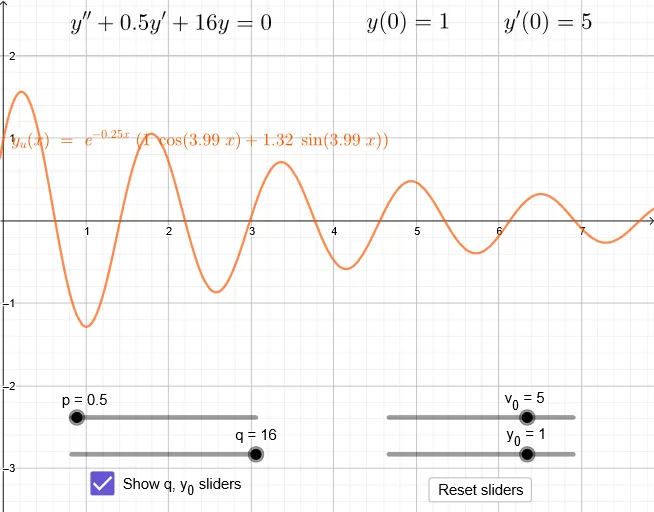
This example demonstrates damped harmonic motion. It involves differential equations and trigonometric functions from calculus. By constructing objects like function f, slider animation button1, and loci C_c, C_u, the dynamic process of harmonic motion is clearly illustrated. Suitable for high school physics and mathematics courses.
GeoGebra Commands & Parameters
Numeric y_0(1)Numeric v_0(5)Numeric p(0.5)Numeric q(16)((-p) - sqrt(p^(2) - (4 * q))) / 2((-p) + sqrt(p^(2) - (4 * q))) / 2((-v_0) + (l_1 * y_0)) / (l_1 - l_2)(v_0 - (l_2 * y_0)) / (l_1 - l_2)((-p)) / 2sqrt((4 * q) - p^(2)) / 2y_v(x) = (C_1 * ℯ^((l_1 * x))) + (C_2 * ℯ^((l_2 * x)))Boolean d(true)f(x) = x^(2) + (p * x) + 16(y_0 * p / 2) + v_0(v_0 - (y_0 * a)) / by_u(x) = (ℯ^((a * x)) * ((y_0 * cos((b * x))) + (C_u * sin((b * x)))))y_c(x) = (ℯ^((l_1 * x)) * (y_0 + (C_c * x)))5
AI Drawing Prompt Reference
Draw a damped harmonic motion graph, including a quadratic function f(x) = x^2 + 0.5x + 16 with initial conditions y_0=1 and v_0=5. Adjust parameters p and q to observe changes in functions y_v(x) and y_u(x), where y_v(x) = (C_1 * e^(l_1 * x)) + (C_2 * e^(l_2 * x)) and y_u(x) = (e^(a * x) * (y_0 * cos(b * x) + C_u * sin(b * x))). Also, plot y_c(x) = (e^(l_1 * x) * (y_0 + C_c * x)) and observe its changes over time.
The prompt above was compiled from the original drawing commands and is for reference only.