
Half-life Determination: Exponential Functions and Geometric Construction
Loading the math board and drawing, please wait…
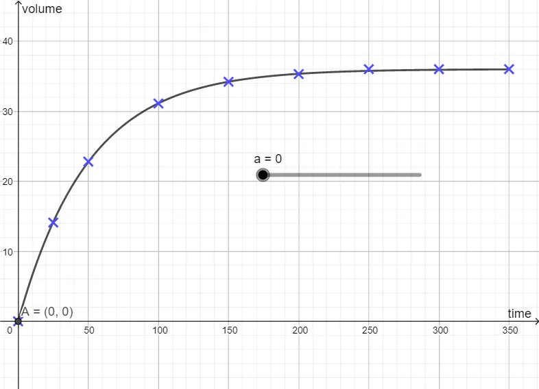
This example demonstrates the concept of half-life using exponential function models. Key mathematical concepts include exponential growth and decay patterns. Construction involves using GeoGebra commands to create function graphs, mark critical points, and analyze half-life parameters. Suitable for high school students learning exponential function applications and geometric construction techniques.
GeoGebra Commands & Parameters
f(x) = If[0 ≤ x ≤ 350, 36 - (36 * ℯ^((-0.02 * x)))](0, 0)(25, 14.1)(50, 22.8)(100, 31.1)(150, 34.2)(200, 35.3)Numeric a(0)(250, 36)(300, 36)(350, 36)(a, f(a))
AI Drawing Prompt Reference
Create a coordinate-plane graph of an exponential decay model. Plot the curve of f(x)=36-(36·e^(-0.02x)) over the interval 0 ≤ x ≤ 350. Mark the key points (0,0), (25,14.1), (50,22.8), (100,31.1), (150,34.2), (200,35.3), and also the points approaching the plateau (250,36), (300,36), (350,36). Then indicate a parameter-based point on the curve of the form (a, f(a)), using a chosen numerical value a to represent the half-life estimate, and connect it only through the function relationship y=f(a).
The prompt above was compiled from the original drawing commands and is for reference only.