
Half-Life Determination (1)
Loading the math board and drawing, please wait…
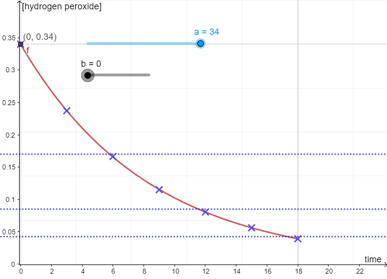
This example demonstrates how to determine half-life through graphical methods, visually showcasing exponential decay processes. Key math concepts include exponential functions, step functions, binomial distribution, trigonometry, quadratic functions, and equations. Construction highlights involve GeoGebra commands/objects like a, f, g, h, p, b, C, D, E, F, G, H, I, B for building decay curves and interactive demonstrations. Suitable for high school and above, aiding quantitative analysis of radioactive decay or similar exponential phenomena.
GeoGebra Commands & Parameters
Numeric a(34)f(x) = If[0 ≤ x ≤ 18, (a / 100 * ℯ^((-0.12 * x)))]y = 0.17y = 0.085y = 0.0425Numeric b(0)(0, 0.34)(3, 0.2372)(6, 0.1665)(12, 0.0806)(18, 0.0392)(9, 0.115)(15, 0.0562)(b, f(b))
AI Drawing Prompt Reference
Create a graph for determining half-life using an exponential decay curve. Use parameter a=34 and draw a function y=f(x) defined for 0≤x≤18 as y = (a/100)·e^(-0.12x). On the same coordinate system, add three horizontal guide lines at y=0.17, y=0.085, and y=0.0425 to represent successive halving levels. Plot key points to visualize the decay, including (0,0.34), (3,0.2372), (6,0.1665), (12,0.0806), and (18,0.0392), and also include points on/at the curve such as (9,0.115) and (15,0.0562). Indicate the idea of solving for a value b where b = f(b) by relating b to the curve.
The prompt above was compiled from the original drawing commands and is for reference only.