
Graphs of Cubic, Quadratic and Linear Functions
Loading the math board and drawing, please wait…
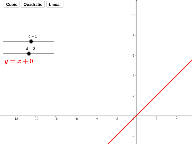
This example uses sliders to graph cubic, quadratic, and linear functions. It demonstrates the basic properties of polynomial functions, including the direction of opening, axis of symmetry, and zeros. By adjusting the sliders, you can observe changes in the function's graph. The GeoGebra commands used include a, b, c, d, f, g, h, e, and k. Suitable for high school mathematics education and learning.
GeoGebra Commands & Parameters
Numeric a(0)Numeric b(0)Numeric c(1)Numeric d(0)Boolean f(false)g(x) = (a * x^(3)) + (b * x^(2)) + (c * x) + dBoolean h(false)y = (c * x) + dy = (b * x^(2)) + (c * x) + d
AI Drawing Prompt Reference
Draw the graph of a cubic function, a quadratic function, and a linear function. Use sliders to adjust the coefficients of the cubic function and observe the changes in the graph. Then, draw the graphs of the quadratic and linear functions, paying attention to their relationship with the cubic function graph.
The prompt above was compiled from the original drawing commands and is for reference only.