Graphing the Normal Curve with Mean and Standard Deviation

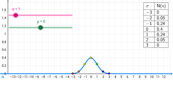
This GeoGebra example demonstrates how to graph a normal distribution curve based on a specified mean (μ) and standard deviation (σ), highlighting its symmetric bell-shaped form. The core mathematical concepts include the normal probability density function, how the mean shifts the curve horizontally, how the standard deviation affects its spread, and the relationship between variance and standard deviation. Construction details: the example uses Text and TableText commands to create dynamic labels and data tables, sliders or input fields to control μ and σ, and multiple point objects (such as A, B, C, etc.) along with a list (list1) to sample points on the curve, ultimately producing a smooth normal curve. This resource is suitable for high school and introductory college statistics courses, helping students visualize how changing parameters alters the distribution, and can also serve as a tool for teaching probability density functions.