
Power of the Test Demonstration
Loading the math board and drawing, please wait…
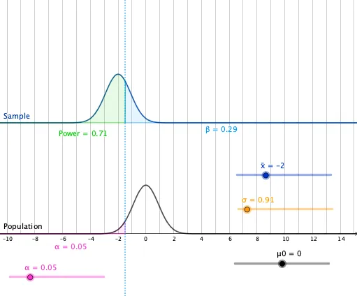
This example demonstrates the concept of the power of a statistical test, visually showing how changes in parameters affect the power. It involves core mathematical concepts like normal distribution, test power, significance level, and critical value. The construction uses commands such as Normal, InverseNormal, IntegralBetween, and Integral, along with objects like μ0, xbar, σ, f, g, α, z_, h, line1, c, a, and b. It is suitable for high school students and above, particularly those learning statistics.
GeoGebra Commands & Parameters
Normal(μ0, σ, x, false) → fInverseNormal(μ0, σ, α) → z_*IntegralBetween(g, line1, -100, z_*) → cIntegral(Normal[μ0, σ, x, false], -20, z_*) → aIntegralBetween(g, line1, z_*, 20) → b
AI Drawing Prompt Reference
Draw a normal distribution curve representing the null hypothesis mean μ0 and standard deviation σ. Then, plot the z_ value corresponding to the significance level α, and calculate and display the area c to the left of z_, and the area b from z_ to 20.
The prompt above was compiled from the original drawing commands and is for reference only.