
Graphing Parametric Equations
Loading the math board and drawing, please wait…
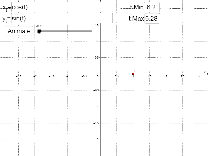
This example demonstrates how to graph parametric equations in a 2D coordinate system. Key math concepts include parametric equations, coordinate geometry, and function graphing. It utilizes GeoGebra commands like Textfield, Curve, Sequence, and Segment to construct the parametric curves. Suitable for high school mathematics education and learning applications of parametric equations.
GeoGebra Commands & Parameters
Textfield(f) → inputBox1Textfield(g) → inputBox2CurveCartesian(f(t), g(t), t, tMin, tMax) → bCurveCartesian(f(t), g(t), t, tMin, a) → eTextfield(tMin) → inputBox3Textfield(tMax) → inputBox4Sequence(tMin + (tMax - tMin) / 10 + ((k * (tMax - tMin))) / 5, k, 0, 4) → l1, {-5.0236814692820415, -2.511044407846124, 0.0015926535897934357, 2.514229715025711, 5.026866776461628}Segment(e(l1(2)), e(l1(2) + 0.0001)) → iSegment(e(l1(1)), e(l1(1) + 0.0001)) → hSegment(e(l1(3)), e(l1(3) + 0.0001)) → jSegment(e(l1(4)), e(l1(4) + 0.0001)) → kSegment(e(l1(5)), e(l1(5) + 0.0001)) → l