
Graphing Linear Equations by SuperPisTeacher
Loading the math board and drawing, please wait…
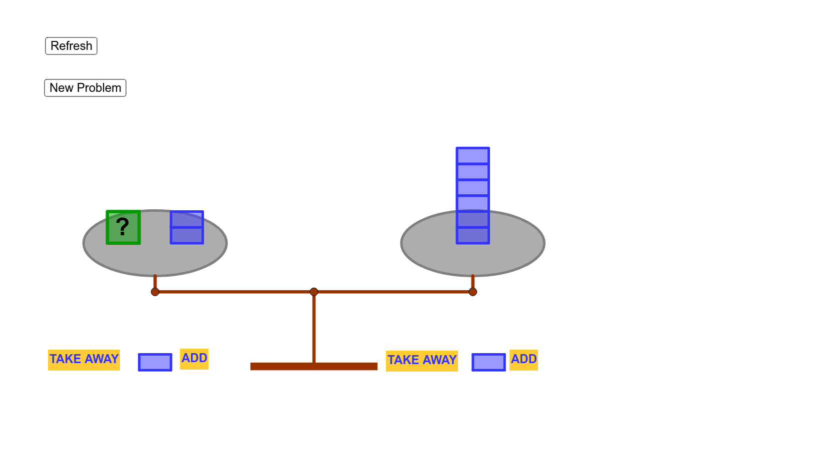
This example demonstrates the graphical representation of linear equations. Key mathematical concepts include equations, roots, and number properties. Using GeoGebra commands such as If, Polygon, and Ellipse, the graphical representation of the equation is constructed. Suitable for beginners to learn the geometric representation of equations.
GeoGebra Commands & Parameters
If(u + L ≟ R, 0, If[u + L ≥ R, -1, 1]) → BPolygon((-6.5, B), (-5.5, B), 4) → poly1Ellipse((-3, B), (-7, B), 2.25) → cEllipse((3, (-B)), (7, (-B)), 2.25) → dSegment((-5, B), (-5, -3)) → aIntersect(c, a) → A,Segment((5, (-B)), (5, -3)) → bIntersect(d, b) → C,Segment(A, A') → eSegment(C, C') → fSegment(A', C') → gIntersect(yAxis, g) → DPoint(yAxis) → ESegment(D, E) → hPolygon(F, G, H, I) → poly3, f_1, g_1, h_1, i_1Midpoint(J, M) → OPolygon((-5.5, -4), (-4.5, -4), (-4.5, -3.5), (-5.5, -3.5)) → poly2, i, j, k, mSequence(Polygon[(4.5, (-B) - 0.5 + t / 2), (5.5, (-B) - 0.5 + t / 2), (5.5, (-B) + t / 2), (4.5, (-B) + t / 2)], t, 1, R, 1) → list2Sequence(Polygon[(-4.5, B - 0.5 + t / 2), (-3.5, B - 0.5 + t / 2), (-3.5, B + t / 2), (-4.5, B + t / 2)], t, 1, L, 1) → list1Polygon((-5.5, -4), (-4.5, -4), (-4.5, -3.5), (-5.5, -3.5)) → poly2_1, i_2, j_1, k_1, m_1Polygon((5, -4), (6, -4), (6, -3.5), (5, -3.5)) → poly4, n, p, q, s