
Graph the Derivative Function
Loading the math board and drawing, please wait…
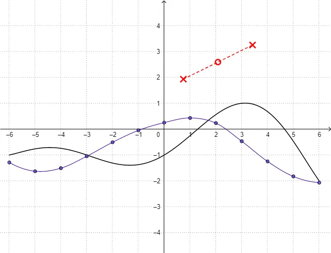
This example demonstrates how to graph the derivative function of a given function, involving core math concepts like derivatives, function graphs, and rates of change. Key GeoGebra commands used include Sequence, Corner, FitPoly, Function, Segment, and Point for constructing the graph, suitable for high school calculus students or teachers.
GeoGebra Commands & Parameters
Sequence((i, Random[-2, 3] + (0 * dummy)), i, -12, 12, 3) → fPointListCorner(1) → panelPt1Corner(4) → panelPt4FitPoly(fPointList, Length[fPointList] - 1) → fFunction(f, -6, 6) → fResFunction(g, -6, 6) → gResSegment((-6, -3.5), (-6, 4.5)) → segASegment((-5, -3.5), (-5, 4.5)) → segBSegment((-4, -3.5), (-4, 4.5)) → segCSegment((-3, -3.5), (-3, 4.5)) → segDSegment((-2, -3.5), (-2, 4.5)) → segESegment((-1, -3.5), (-1, 4.5)) → segFSegment((0, -3.5), (0, 4.5)) → segGSegment((1, -3.5), (1, 4.5)) → segHSegment((2, -3.5), (2, 4.5)) → segISegment((3, -3.5), (3, 4.5)) → segJSegment((4, -3.5), (4, 4.5)) → segKSegment((5, -3.5), (5, 4.5)) → segLSegment((6, -3.5), (6, 4.5)) → segMPoint(segA) → APoint(segB) → BPoint(segC) → CPoint(segD) → DPoint(segE) → EPoint(segF) → FPoint(segG) → GPoint(segH) → HPoint(segI) → IPoint(segJ) → JPoint(segK) → KPoint(segL) → LPoint(segM) → MFitPoly({A, B, C}, 2) → parABCFitPoly({C, D, E}, 2) → parCDEFitPoly({E, F, G}, 2) → parEFGFitPoly({G, H, I}, 2) → parGHIFitPoly({I, J, K}, 2) → parIJKFitPoly({K, L, M}, 2) → parKLMFitPoly({B, C, D}, 2) → parBCDFitPoly({D, E, F}, 2) → parDEFFitPoly({F, G, H}, 2) → parFGHFitPoly({H, I, J}, 2) → parHIJFitPoly({J, K, L}, 2) → parJKLFunction(parABC, x(A), x(B)) → conABFunction((parABC(x) * (1 - (x + 5))) + (parBCD(x) * (x + 5)), -5, -4) → conBCFunction((parBCD(x) * (1 - (x + 4))) + (parCDE(x) * (x + 4)), -4, -3) → conCDFunction((parCDE(x) * (1 - (x + 3))) + (parDEF(x) * (x + 3)), -3, -2) → conDEFunction((parDEF(x) * (1 - (x + 2))) + (parEFG(x) * (x + 2)), -2, -1) → conEFFunction((parEFG(x) * (1 - (x + 1))) + (parFGH(x) * (x + 1)), -1, 0) → conFGFunction((parFGH(x) * (1 - (x + 0))) + (parGHI(x) * (x + 0)), 0, 1) → conGHFunction((parGHI(x) * (1 - (x - 1))) + (parHIJ(x) * (x - 1)), 1, 2) → conHIFunction((parHIJ(x) * (1 - (x - 2))) + (parIJK(x) * (x - 2)), 2, 3) → conIJFunction((parIJK(x) * (1 - (x - 3))) + (parJKL(x) * (x - 3)), 3, 4) → conJKFunction((parJKL(x) * (1 - (x - 4))) + (parKLM(x) * (x - 4)), 4, 5) → conKLFunction(parKLM, 5, 6) → conLMSegment(Q, P) → h
AI Drawing Prompt Reference
Draw the graph of a function and its derivative. First, generate a series of random points and fit them to a polynomial function to plot the function. Then, place multiple horizontal line segments at equal intervals on the x-axis and place a point on each segment. Finally, fit quadratic polynomials to these points and connect them with smooth curves to obtain the derivative graph.
The prompt above was compiled from the original drawing commands and is for reference only.