
Geometric Similarity from a Variable-Parts Perspective by Sybilla Beckmann
Loading the math board and drawing, please wait…
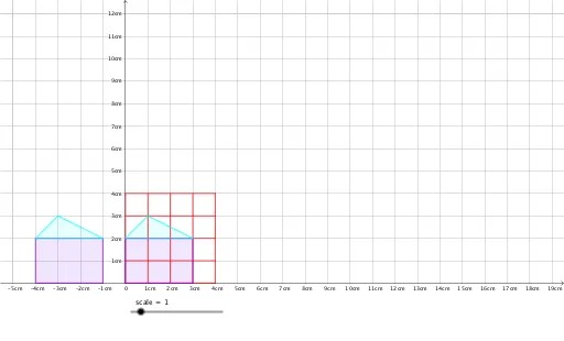
This example demonstrates geometric similarity from a variable-parts perspective, involving concepts like dilation, linear regression, and normal distribution. It uses GeoGebra commands such as Point, Polygon, Ray, Circle, Intersect, Line, and Segment. Suitable for high school and above, it illustrates the integration of geometric transformations and data analysis.
GeoGebra Commands & Parameters
Point(xAxis) → APoint(xAxis) → DPolygon(A, B, C, D) → q1, a, b, c, dPolygon(B, E, C) → t1, c_1, b_1, ePoint(yAxis) → FPoint(xAxis) → GRay(F, G) → gPoint(yAxis) → HRay(F, H) → hCircle(F, f) → kIntersect(g, xAxis) → IIntersect(g, xAxis) → JIntersect(g, xAxis) → KIntersect(k, g) → L,Intersect(k, h, 1) → MCircle(L, f) → pCircle(M, f) → qIntersect(q, h, 2) → NIntersect(p, g, 2) → OCircle(N, f) → rCircle(O, f) → sIntersect(r, h, 2) → PIntersect(s, g, 2) → QCircle(P, f) → tCircle(Q, f) → d_1Intersect(t, h, 2) → RIntersect(d_1, g, 2) → SLine(R, g) → iLine(P, i) → jLine(N, j) → lLine(M, l) → mLine(S, h) → nLine(Q, h) → f_1Line(O, h) → g_1Line(L, h) → h_1Intersect(i, h_1) → TIntersect(i, g_1) → UIntersect(i, f_1) → VIntersect(i, n) → WIntersect(j, n) → ZIntersect(l, n) → A_1Intersect(m, n) → B_1Segment(F, S) → i_1Segment(M, B_1) → j_1Segment(N, A_1) → k_1Segment(P, Z) → l_1Segment(R, W) → m_1Segment(F, R) → n_1Segment(L, T) → p_1Segment(O, U) → q_1Segment(Q, V) → r_1Segment(S, W) → s_1Intersect(k_1, r_1) → C_1Polygon(F, N, C_1, Q) → q2, f_2, n_2, c_2, q_2Intersect(l_1, p_1) → D_1Polygon(N, D_1, C_1) → t2, c_3, n_3, d_2