
Geometric Distribution & Expected Value
Loading the math board and drawing, please wait…
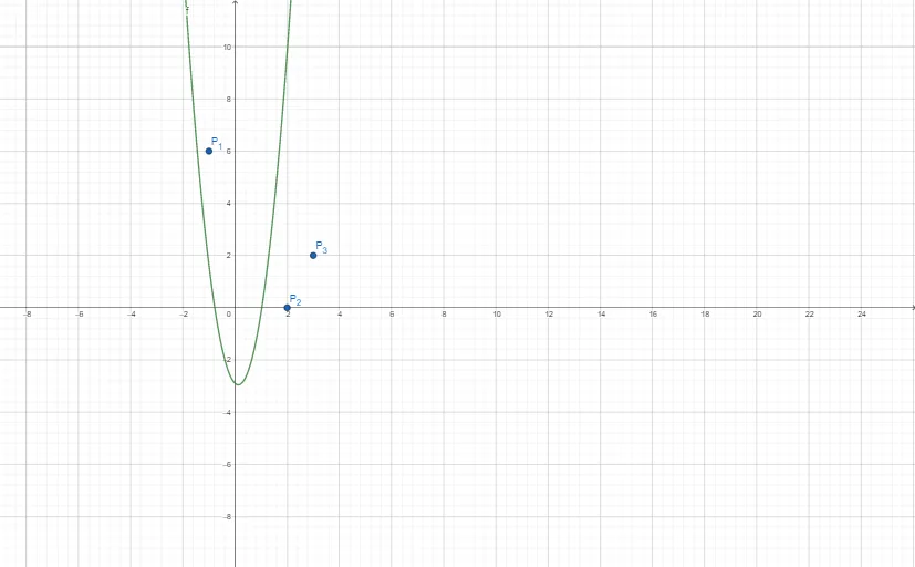
This example demonstrates the dynamic visualization of geometric distribution probability calculations and expected value computation using GeoGebra. Key math concepts include geometric distribution, expected value, random experiments, line segment length calculation, and multiplication principle. The construction leverages GeoGebra commands/objects like a, b, c, P₁, P₂, P₃, f for parametric modeling. Suitable for high school probability & statistics courses to understand discrete random variable properties and expectation calculation.
GeoGebra Commands & Parameters
Numeric a(-2.9)Numeric b(-0.9)Numeric c(3.63)(-1, 6)(2, 0)(3, 2)f(x) = (c * x^(2)) + (b * x) + a
AI Drawing Prompt Reference
Draw a function graph representing a quadratic function with coefficients determined by three values ranging from -2.9 to -0.9 to 3.63, passing through points (-1, 6) and (2, 0), and another point (3, 2) to visualize geometric distribution probability calculations and expected value dynamically.
The prompt above was compiled from the original drawing commands and is for reference only.