
GeoGebra Demonstration of Additive Property of Definite Integral
Loading the math board and drawing, please wait…
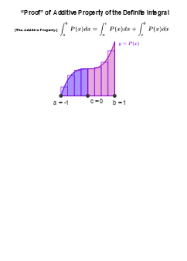
This example dynamically demonstrates the additive property of definite integrals using GeoGebra, showing that the integral over a combined interval equals the sum of integrals over subintervals. Core math concepts include definite integrals, function graphs, interval division, and vector operations. Construction highlights involve commands like Sequence, Integral, Point, Line, Vector, etc., as per the summary to build function graphs, segment lines, and compute integrals. Suitable for high school and above to understand the geometric meaning of the additive property theorem.
GeoGebra Commands & Parameters
Sequence(1, n) → N1Sequence(0, n) → N0Zip(a - dx / 2 + (k * dx), k, N1) → c_*Zip(a + (k * dx), k, N0) → x_*IndexOf(1, Findc) → c_#Integral(P, a, c) → IPacIntegral(P, c, b) → IPcbIntegral(P, a, b) → IPabTextfield(P) → inputBox1Point(yAxis) → DPoint(yAxis) → ELine(D, E) → XaxisLine(Ypt, Xaxis) → YaxisVector(G, J) → uVector(I, F) → vVector(H, K) → wSegment(F, K) → fSegment(F, J) → hSegment(I, H) → iSegment(G, I) → jIntegral(αP, a, b) → IαPabLine(M, Yaxis) → Y2axisVector(J, αs_a) → eVector(K, αs_b) → dSegment(αs_a, αs_b) → gSegment(J, K) → mSegment(G, H) → pTextfield(Q) → InputBox1Integral(Q, a, b) → IQabIntegral(P(x) + Q(x), a, b) → IPQabLine(O, Xaxis) → qVector(G, SQa) → rVector(H, SQb) → sSegment(SQb, SQa) → tVector(K, SPQb) → u_1Vector(SQb, SPQb) → v_1Vector(SQa, SPQa) → w_1Segment(SPQb, SPQa) → f_1Vector(SQb, SQb1) → a_1Segment(SPQb, SQb1) → g_1Segment(SQb1, SPQa) → h_1Vector(J, SQb1) → b_1Point(f_1) → RZip((0, a + (k * dx)), k, N0) → x_1Zip(Sum[Pcdx_*, k], k, N0) → SPcdx_*Zip(Sum[αPxdx_*, k], k, N0) → SαPcdx_*Zip((x(Ypt), sp), sp, SPcdx_*) → SptPcdx_*Zip(Vector[A, B], A, x_1, B, SptPcdx_*) → vecSP_*Zip((x(M), sp), sp, SαPcdx_*) → SptαPcdx_*Zip(Vector[A, B], A, SptPcdx_*, B, SptαPcdx_*) → vecSαP_*TableText(Transpose[{Join[{{"c_k"}, c_*}], Join[{{"P(c_k)Δx"}, Pcdx_*}], Join[{{"αP(c_k)Δx"}, αPxdx_*}]}], "|_cc") → TableIRectangleSum(P, y(G), y(H), n, 1 / 2) → GrMidEstIntPRectangleSum((α * P(x)), y(G), y(H), n, 1 / 2) → GrMidestIntαPZip(Sum[Qcdx_*, k], k, N0) → SQcdx_*Zip((x(M), sp), sp, SQcdx_*) → SptQcdx_*Zip(Vector[A, B], A, x_1, B, SptQcdx_*) → vecSQ_*Zip(Sum[PQcdx_*, k], k, N0) → SPQcdx_*Zip((x(O), sp), sp, SPQcdx_*) → SptPQcdx_*Zip(Vector[A, B], A, SptPcdx_*, B, SptPQcdx_*) → vecSP2PQ_*Zip(Vector[A, B], A, SptQcdx_*, B, SptPQcdx_*) → vecSQ2PQ_*RectangleSum(Q, y(G), y(H), n, 1 / 2) → GrMidEstIntQRectangleSum(PQ, y(G), y(H), n, 1 / 2) → GrMidEstIntPQZip((x(O), sp), sp, SQcdx_*) → SptQ'cdx_*Zip(Vector[A, B], A, SptQcdx_*, B, SptQ'cdx_*) → vecSQ'_*Zip((x(O), sp), sp, SPcdx_* + GrMidEstIntQ) → SptP'cdx_*Zip(Vector[A, B], A, SptPcdx_*, B, SptP'cdx_*) → vecSP'_*Vector(G, M_0) → d_1Vector(G, O_0) → e_1TableText(Transpose[{Join[{{"c_k"}, c_*}], Join[{{"P(c_k)Δx"}, Pcdx_*}]}], "|_cc") → TablePElement(x_*, c_# - 1) → c1RectangleSum(P, y(G), c1, c_# - 2, 1 / 2) → GrMidEstIntP1Element(x_*, c_#) → c2RectangleSum(P, c2, y(H), n - c_# + 1, 1 / 2) → GrMidEstIntP2First(c_*, c_# - 2) → c1_*Last(c_*, n - c_# + 1) → c2_*Join({c1_*, {c}, c2_*}) → ca_*Zip(Sum[Pcadx_*, k], k, N0) → SPcadx_*Zip((x(Ypt), sp), sp, SPcadx_*) → SptPcadx_*Zip(Vector[A, B], A, x_1, B, SptPcadx_*) → vecSPa_*
AI Drawing Prompt Reference
Draw a function graph to demonstrate the additive property of definite integrals. Mark three intervals [a, c], [c, b], and [a, b] on the x-axis, and calculate and display the definite integral values for each interval. Use geometric shapes and vector operations to visually show that the integral over [a, b] equals the sum of the integrals over [a, c] and [c, b]. Start by plotting the function curve and coordinate axes, then label key points and lines, and finally use vectors to represent the integral regions to complete the construction.
The prompt above was compiled from the original drawing commands and is for reference only.