
Function Loupe I (Slope)
Loading the math board and drawing, please wait…
In collections
ICME 13, TSG 16: A visual approach to calculus
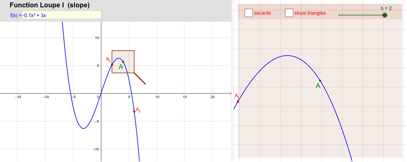
This example demonstrates how to observe the slope of a function using GeoGebra. Key mathematical concepts include functions, derivatives, and limits. By constructing triangles, segments, and using slider animations, users can dynamically observe the slope changes at different points on the function. Suitable for high school mathematics education and learning.
GeoGebra Commands & Parameters
Textfield(f) → Textfeld1Point(f) → APolygon(A + ((-h), (-h)), A + (h, (-h)), A + (h, h), A + ((-h), h)) → Lupe, i, j, k, lPolygon(A, Ar, A_r) → StDreieckre_1, a, g, mPolygon(Al, A_l, A) → StDreieckli, n, p, qSegment(A_l, Al) → bSegment(Al, A) → cSegment(A, Ar) → dSegment(A + (h, (-h)), A + (2 * (h, (-h)))) → griff1Line(A_l, A) → sek_lLine(A, A_r) → sek_rSegment(A + (min, (-min)), A + (2 * (min, (-min)))) → griff2If(h > min, griff1, griff2) → griffPolygon(F, G, D, E) → Vieleck4, f_2, g_2, d_2, e_2
AI Drawing Prompt Reference
Draw a function curve with a movable point on it. Around this point, construct a square magnifying glass whose side length is controlled by a slider. Inside the glass, draw two secant lines through the point to nearby left and right points, forming two small triangles to illustrate the slopes. Outside the glass, extend a segment from the point parallel to the secant, with length varying by the slider, to indicate the slope direction. The whole figure updates dynamically with the slider, showing how the slope changes near the point.
The prompt above was compiled from the original drawing commands and is for reference only.