
Function Calculus Magic Machine
Loading the math board and drawing, please wait…
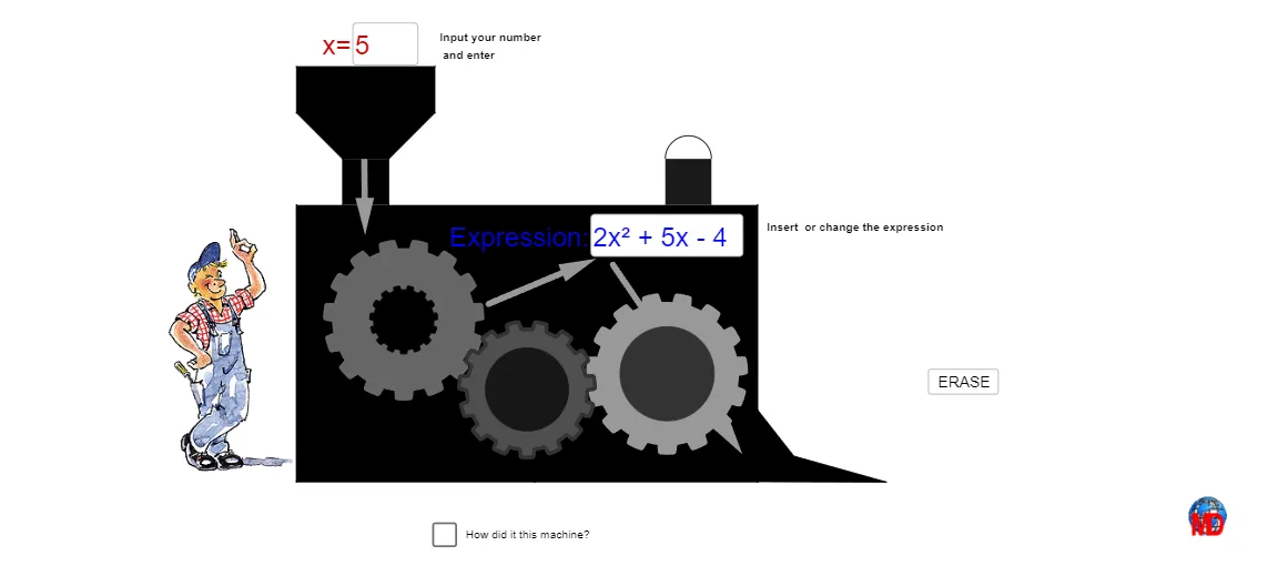
This example demonstrates the dynamic process of function calculus, involving concepts such as derivatives, integrals, and limits. Using GeoGebra commands like CurveCartesian, Circle, and Polygon, it provides an intuitive view of function changes. Suitable for high school and above students learning calculus.
GeoGebra Commands & Parameters
CurveCartesian(x(A) + ((r * (a + (1 / b * tanh((b * sin((n * t) + v)))))) * cos(t + v)), y(A) + ((r * (a + (1 / b * tanh((b * sin((n * t) + v)))))) * sin(t + v)), t, 0, 6.28319) → cCurveCartesian(x(B) + ((R * (a + (1 / b * tanh((b * sin((n * t) - v)))))) * cos(t - v)), y(B) + ((R * (a + (1 / b * tanh((b * sin((n * t) - v)))))) * sin(t - v)), t, 0, 6.28319) → dCircle(B, R + 0.9) → eCircle(A, r + 0.9) → gCircle(A, r + 0.9) → hCurveCartesian(x(A) + ((r * (a + (1 / b * tanh((b * sin((n * t) + v)))))) * cos(t + v)), y(A) + ((r * (a + (1 / b * tanh((b * sin((n * t) + v)))))) * sin(t + v)), t, 0, 6.28319) → iCurveCartesian(x(C) + ((R * (a + (1 / b * tanh((b * sin((n * t) - v)))))) * cos(t - v)), y(C) + ((R * (a + (1 / b * tanh((b * sin((n * t) - v)))))) * sin(t - v)), t, 0, 6.28319) → jCurveCartesian(x(C) + ((r / 2 * (a + (1 / b * tanh((b * sin((n * t) + v)))))) * cos(t + v)), y(C) + ((r / 2 * (a + (1 / b * tanh((b * sin((n * t) + v)))))) * sin(t + v)), t, 0, 6.28319) → oPolygon(D, E, F, G) → poly1, d_1, e_1, f_1, g_1Point(g_1) → HPoint(g_1) → IPolygon(H, I, J, K) → poly2, h_1, i_1, j_1, kPolygon(L, K, J, M) → poly3, l, k_1, j_2, mPoint(f_1) → NPolygon(N, O, P, F) → poly4, n_1, o_1, p, f_2Textfield(s) → ChampTexte1Vector(Q, S) → uTextfield(f) → ChampTexte2Vector(U, V) → wVector(W, Z) → zPolygon(C_1, M, L, D_1) → poly5, c_1, m_1, l_1, d_2Polygon(E_1, F_1, G_1, H_1) → poly6, e_2, f_3, g_2, h_2Semicircle(F_1, G_1) → qMod(v / °, 2) → t_1Semicircle(F_1, G_1) → p_1Segment(A_1, B_1) → a_1Coefficients(f) → liste1Polynomial(f) → ffCoefficients(ff) → mmElement(liste1, 1) → aaElement(liste1, 2) → bbElement(liste1, 3) → cc
AI Drawing Prompt Reference
Create a visual representation of function calculus dynamics. Start with two base points as centers, draw two closed curves defined by parametric equations with hyperbolic tangent modulation, creating wavy edges. Add a large auxiliary circle around one center and two concentric circles around the other. From a third point, draw a similar curve with half radius. Connect several key points with polygons to form quadrilateral regions, and add semicircles on some edges. Include two text input fields and several vector arrows to indicate relationships between functions, derivatives, and integrals. The overall layout shows an intuitive visualization of function transformations.
The prompt above was compiled from the original drawing commands and is for reference only.