
Fubini's Theorem Visualization
Loading the math board and drawing, please wait…
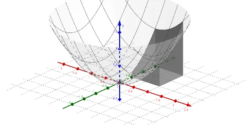
This example dynamically demonstrates Fubini's theorem, illustrating the interchange of order in double integrals. Key math concepts include integration, volume, solids of revolution, and coordinate transformations. Construction highlights involve Surface, Segment, CurveCartesian commands for modeling regions and solids, with Textfield and Eingabefeld objects for parameterized interaction. Suitable for high school and above students, and calculus instruction.
GeoGebra Commands & Parameters
Textfield(f) → Eingabefeld1Textfield(vonx) → Eingabefeld2Textfield(bisx) → Eingabefeld3Textfield(vony) → Eingabefeld4Textfield(bisy) → Eingabefeld5Surface(u, vony, (w * f(u, vony)), u, vonx, bisx, w, 0, 1) → O_1Surface(bisx, u, (w * f(bisx, u)), u, vony, bisy, w, 0, 1) → O_2Surface(u, bisy, (w * f(u, bisy)), u, vonx, bisx, w, 0, 1) → O_3Surface(vonx, u, (w * f(vonx, u)), u, vony, bisy, w, 0, 1) → O_4Segment((vonx, a, 0), (bisx, a, 0)) → s_1Segment((bisx, a, 0), (bisx, a, f(bisx, a))) → s_2Segment((vonx, a, 0), (vonx, a, f(vonx, a))) → s_3Segment((b, a, 0), (b, a, f(b, a))) → sCurveCartesian(t, a, f(t, a), t, vonx, bisx) → kurvSurface(u, a, (w * f(u, a)), u, vonx, bisx, w, 0, 1) → O_ySurface(u, (0.99 * a), (w * f(u, a)), u, vonx, b, w, 0, 1) → O1_y