
Fruit Fly Population Function Modeling with GeoGebra
Loading the math board and drawing, please wait…
In collections
CCSS IP Math I Unit 4 Lesson 2
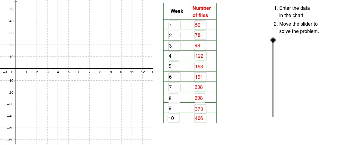
This GeoGebra example models fruit fly population change over 10 weeks, linking tabular data to graphical function representation. It demonstrates function modeling (exponential or sinusoidal), sequences, coordinate geometry, and tangent line rate-of-change analysis. Constructed using Textfield, Polygon, Sequence, and Segment commands, it generates structured point sets (A1-A11, B1-B11, C1-C11, D1-D7) to visualize population trends and geometric relationships. Ideal for high school mathematical modeling, algebra, trigonometry, and real-world data interpretation units.
GeoGebra Commands & Parameters
Textfield(A2) → InA2Textfield(A3) → InA3Textfield(A4) → InA4Textfield(A5) → InA5Textfield(A6) → InA6Textfield(A7) → InA7Textfield(A8) → InA8Textfield(A9) → InA9Textfield(A10) → InA10Textfield(A11) → InA11Textfield(B2) → InB2Textfield(B3) → InB3Textfield(B4) → InB4Textfield(B5) → InB5Textfield(B6) → InB6Textfield(B7) → InB7Textfield(B8) → InB8Textfield(B9) → InB9Textfield(B10) → InB10Textfield(B11) → InB11Polygon((13, y(Corner[1])), Corner[2], Corner[3], (13, y(Corner[4]))) → poly1, b, c, d, eSequence(Segment[(14, (-46) + (8.7 * i)), (19, (-46) + (8.7 * i))], i, 0, 10) → CrossList1Segment((14, 55), (19, 55)) → Top1Segment((19, 55), (21.5, 55)) → Top2Segment((21.5, 55), (24, 55)) → Top3Segment((21.5, -46.256410256410255), (21.5, 54.743589743589745)) → Side2Segment((24, -46), (24, 55)) → Side3Sequence(Segment[(21.5, (-46) + (8.7 * i)), (24, (-46) + (8.7 * i))], i, 0, 10) → CrossList3Sequence(Segment[(19, (-46) + (8.7 * i)), (21.5, (-46) + (8.7 * i))], i, 0, 10) → CrossList2Sequence(Segment[(14 + (2.5 * i), (-46)), (14 + (2.5 * i), 55)], i, 0, 2) → SideList1