
Free Vibrations Without Damping
Loading the math board and drawing, please wait…
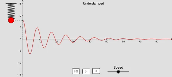
This example demonstrates the physical phenomenon of free vibrations without damping. Core mathematical concepts include differential equations and coordinate geometry. Using GeoGebra commands such as If, Element, Segment, Textfield, etc., the vibration curve can be constructed. Suitable for high school physics and mathematics education.
GeoGebra Commands & Parameters
If(c < sqrt(((4 * m) * k)), ((((-c) * sqrt((-c^(2)) + ((4 * k) * m))) * a) + (((-2 * m) * sqrt((-c^(2)) + ((4 * k) * m))) * b)) / (c^(2) - ((4 * k) * m)), If[c > sqrt(((4 * m) * k)), (((c^(2) - ((4 * k) * m) + (c * sqrt(c^(2) - ((4 * k) * m)))) * a) + (((2 * m) * sqrt(c^(2) - ((4 * k) * m))) * b)) / ((2 * c^(2)) - ((8 * k) * m)), ((a * c) + ((2 * b) * m)) / ((2 * m))]) → c_2If(c < sqrt(((4 * m) * k)), a, If[c > sqrt(((4 * m) * k)), (((c^(2) - ((4 * k) * m) - (c * sqrt(c^(2) - ((4 * k) * m)))) * a) + (((-2 * m) * sqrt(c^(2) - ((4 * k) * m))) * b)) / ((2 * c^(2)) - ((8 * k) * m)), a]) → c_1If(c < sqrt(((4 * m) * k)), 1, If[c > sqrt(((4 * m) * k)), 2, 3]) → indexElement(List, index) → SolutionSegment(PS, PS + (0, 0.5)) → endSegment(C1, C2) → PlataformSegment(A, A') → LevelSegment((t, 0), A') → LevelTimeTextfield(a) → InputBox1Textfield(b) → InputBox2LaTeX(ω_0, true, true) → text1Textfield(m) → InputBox3Textfield(k) → InputBox4Element(Cases, index) → MotionTextfield(c) → InputBox7CurveCartesian((2 * sin((((9 * 2) * π) * (j - y_1) / y_l))) + x(B), j, j, y_1, y_0) → S
AI Drawing Prompt Reference
Create a diagram illustrating free vibrations without damping. It shows a horizontal platform with a mass attached to a spring above it, moving vertically. Below the platform, a sinusoidal vibration curve is plotted over time. Several input boxes are present for adjusting parameters like mass, spring stiffness, damping coefficient, and initial conditions. Depending on these values, the curve displays three cases: underdamped (oscillatory decay), overdamped (slow return), and critically damped (fast return to equilibrium). Reference lines for equilibrium position and initial displacement are included, along with a time axis. The layout is clear and suitable for physics education.
The prompt above was compiled from the original drawing commands and is for reference only.