
Fraction Division 5: x ÷ a/b (Quotitive) Visualized
Loading the math board and drawing, please wait…
In collections
Primary School Mathematics Collection
Division of Fractions
Division of Fractions
Division of Fractions
Fraction Division
Fraction Division
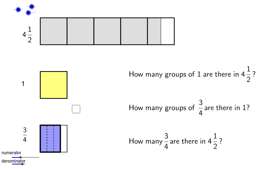
This GeoGebra example dynamically visualizes the quotitive (measurement) division of fractions, demonstrating that x ÷ a/b = x × b/a. Building on the fundamental fact 1 ÷ a/b = b/a, it transforms the abstract algebraic identity into an intuitive area or length partitioning process. The core mathematical concepts include fraction division, reciprocals, the distinction between quotitive and partitive division, and the inverse relationship between multiplication and division. In terms of construction, the example employs GeoGebra commands such as Point, Segment, Polygon, Sequence, If, and FractionText, with objects including a, b, gcd, A, B, C, D, E, F, G, and others. By adjusting parameters a, b, and x, learners can see how many groups of size a/b fit into x, reinforcing the 'how many groups' interpretation. This resource is suitable for upper elementary to middle school students learning fraction operations, and serves as an effective classroom demonstration tool to help students grasp the computational rule through geometric reasoning, overcoming the abstraction barrier of symbolic manipulation.
GeoGebra Commands & Parameters
Point(Segment[(x(E) + 0.1, y(E)), (x(E) + 1, y(E))]) → GPoint(Segment[(x(D) + 0.1, y(D)), (x(D) + 0.5, y(D))]) → FMin(round((x(G) - x(E)) / 0.1), (2 * a')) → b'Max(Sequence[If[(Mod[(a * a'), i] ≤ 0) ∧ (Mod[b', i] ≤ 0), i, 1], i, 1, Min[(a * a'), b']]) → gcdSegment((0, 1), (x(A), y(A))) → f_1Segment(A, (x(A) + a, y(A))) → lSegment((x(A), y(A) + w), (x(A) + a, y(A) + w)) → mSegment(A, (x(A), y(A) + w)) → nSegment((x(A) + 9, y(A)), (x(A) + 9, y(A) + w)) → pSegment((x(A) + 8, y(A)), (x(A) + 8, y(A) + w)) → qSegment((x(A) + 7, y(A)), (x(A) + 7, y(A) + w)) → rSegment((x(A) + 6, y(A)), (x(A) + 6, y(A) + w)) → tSegment((x(A) + 5, y(A)), (x(A) + 5, y(A) + w)) → a_1Segment((x(A) + 4, y(A)), (x(A) + 4, y(A) + w)) → b_1Segment((x(A) + 3, y(A)), (x(A) + 3, y(A) + w)) → c_1Segment((x(A) + 2, y(A)), (x(A) + 2, y(A) + w)) → d_1Segment((x(A) + 10, y(A)), (x(A) + 10, y(A) + w)) → g_1Segment((x(A) + 11, y(A)), (x(A) + 11, y(A) + w)) → h_1Segment((x(A) + 12, y(A)), (x(A) + 12, y(A) + w)) → i_1Segment((x(B) + b' / a', y(B)), (x(B) + a, y(B))) → fPoint(f) → CPolygon(B, ((floor((a' * x(C) / b')) * b' / a'), y(B)), ((floor((a' * x(C) / b')) * b' / a'), y(B) + 1), (x(B), y(B) + 1)) → poly2, poly2_1, poly2_2, poly2_3, poly2_4Segment((x(A) + 1, y(A)), (x(A) + 1, y(A) + w)) → eSegment(E, (x(E) + 1, y(E))) → j_1Segment(D, F) → l_1Polygon(B, (x(B) + 1, y(B)), (x(B) + 1, y(B) + 1), (x(B), y(B) + 1)) → poly1, poly1_1, poly1_2, poly1_3, poly1_4Sequence(Segment[(k / a', y(B)), (k / a', y(B) + 1)], k, 1, a' - 1) → list2Sequence(Segment[(k / a', y(B)), (k / a', y(B) + 1)], k, 1, (floor((a' * x(C) / b')) * b') - 1) → list3Segment(((floor((a' * x(C) / b')) * b' / a'), y(B)), C) → hSegment(((floor((a' * x(C) / b')) * b' / a'), y(B) + 1), (x(C), y(C) + 1)) → iSequence(Segment[(k / a', y(B)), (k / a', y(B) + 1)], k, 1, floor((a' * x(C))) - 1) → list4Sequence(Segment[((k * b' / a'), y(B)), ((k * b' / a'), y(B) + 1)], k, 1, floor((a' * x(C) / b')) - 1) → list1Polygon(((floor((a' * x(C) / b')) * b' / a'), y(B)), C, (x(C), y(C) + 1), ((floor((a' * x(C) / b')) * b' / a'), y(B) + 1)) → poly3, poly3_1, poly3_2, poly3_3, poly3_4Polygon(B, (b' / a', y(B)), (b' / a', y(B) + 1), (x(B), y(B) + 1)) → poly4, poly4_1, poly4_2, poly4_3, poly4_4Segment(((floor((a' * x(C) / b')) * b' / a'), y(B)), ((floor((a' * x(C) / b')) * b' / a') + b' / a', y(B))) → bSegment(((floor((a' * x(C) / b')) * b' / a'), y(B) + 1), ((floor((a' * x(C) / b')) * b' / a') + b' / a', y(B) + 1)) → cSegment(((floor((a' * x(C) / b')) * b' / a') + b' / a', y(B)), ((floor((a' * x(C) / b')) * b' / a') + b' / a', y(B) + 1)) → dSequence(Segment[((floor((a' * x(C) / b')) * b' / a') + k / a', y(B)), ((floor((a' * x(C) / b')) * b' / a') + k / a', y(B) + 1)], k, 1, b' - 1) → list5Segment(E, (Min[x(G), x(E) + (0.2 * a')], y(G))) → m_1Segment(D, (x(D) + 0.5, y(D))) → e_1Polygon(A, (x(A) + a, y(A)), (x(A) + a, y(A) + a), (x(A), y(A) + a)) → poly5, a_2, k_1, n_1, p_1Segment((x(C), Min[y(B) + 1, 2.5]), (x(C), 2.5)) → kPolygon((x(B) + 1, y(B)), (x(B) + 2, y(B)), (x(B) + 2, y(B) + 1), (x(B) + 1, y(B) + 1)) → poly6, poly6_4, poly6_1, poly6_2, poly6_3Sequence(Segment[(k / a' + 1, y(B)), (k / a' + 1, y(B) + 1)], k, 1, a' - 1) → list7Sequence(Segment[(j / a', y(A)), (j / a', y(A) + 1)], j, 1, a' - 1) → list6Point(yAxis) → HPolygon(H, H + (number, 0), H + (number, 1), H + (0, 1)) → poly7, h_2, q_1, r_1, s_1If(floor(number) ≟ number, true, false) → integerSequence(Polygon[H + (i, 0), H + (i + 1, 0), H + (i + 1, 1), H + (i, 1)], i, 0, If[integer, floor(number) - 1, floor(number)]) → list8Sequence(Segment[H + (floor(number) + i, 0), H + (floor(number) + i, 1)], i, 1 / j, (j - 1) / j, 1 / j) → list9FractionText(number - floor(number)) → text41If(¬integer, If[g ≟ 0, text41, text42], text40) → text43If(floor(b' / a') ≟ b' / a', true, false) → integer2If(¬integer2, If[floor(b' / a') ≠ 0, text46, text45], text47) → text48Segment(B + (1, 0), B + (1, 1)) → t_1
AI Drawing Prompt Reference
Draw a figure to represent the fraction division x ÷ a/b, where x is a rectangle, and a and b are adjustable parameters. First, draw a rectangle to represent x, then draw a rectangle representing a/b, and observe how many times the a/b rectangle can fit into the x rectangle. By adjusting the values of a and b, you can see how many a/b rectangles fit into x, thereby understanding the meaning of x divided by a/b.
The prompt above was compiled from the original drawing commands and is for reference only.