
Fraction Addition Visualization: Adding Fractions with Polygons and LCM
Loading the math board and drawing, please wait…
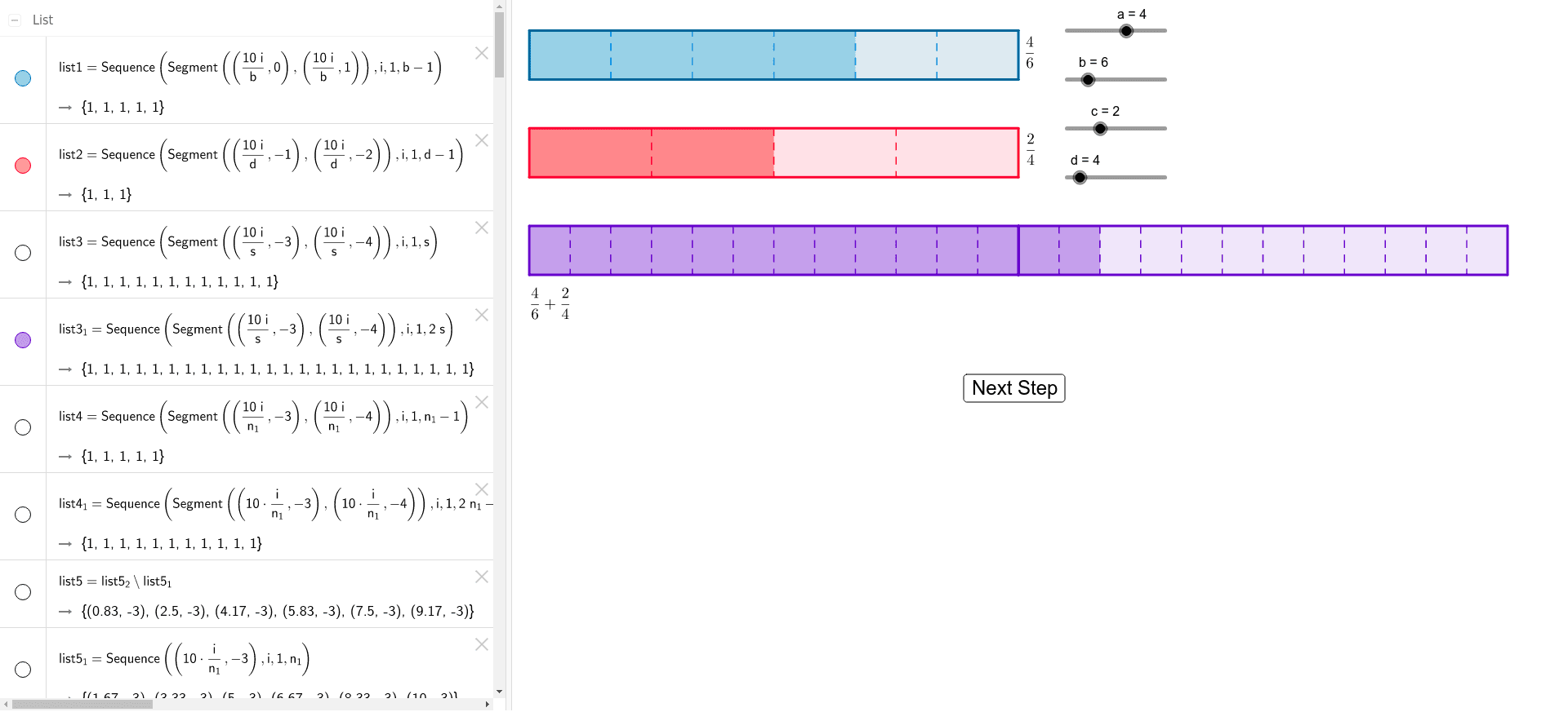
① This GeoGebra example demonstrates fraction addition through a visual area model, using polygons and grid subdivisions to show how fractions with different denominators are combined. ② Core mathematical concepts include fraction addition, least common multiple (LCM), greatest common divisor (GCD), and the correspondence between fractions and geometric area. ③ Construction highlights: from the summary, commands such as Point, Polygon, LCM, Sequence, and GCD are used; multiple polygons (poly1 to poly4) and numerous points (A to P) and segments (a to n) are created. The LCM command finds a common denominator, Sequence generates equal subdivisions, and GCD simplifies the result, making the addition process visually explicit. ④ Suitable for upper elementary to middle school students learning fraction operations, and for teachers demonstrating the link between arithmetic and geometry in a dynamic, interactive way.
GeoGebra Commands & Parameters
Point(Circle[A, 1]) → BPolygon(A, B, C, D) → poly1, a_1, b_1, c_1, d_1Point(Circle[E, 10]) → FPolygon(E, F, G, H) → poly2, e, f, g, hPolygon(I, J, K, L) → poly3, i, j, k, lPolygon(A, B, M, N) → poly4, a_2, b_2, m, nPolygon(H, E, O, P) → poly5, h_1, e_1, o, pPolygon(I, J, Q, R) → poly6, i_1, j_1, q, rLCM(b, d) → sSequence(Segment[(((10 * i)) / b, 0), (((10 * i)) / b, 1)], i, 1, b - 1) → list1Sequence(Segment[(((10 * i)) / d, -1), (((10 * i)) / d, -2)], i, 1, d - 1) → list2GCD(g_1, s) → l_1Polygon(K, L, T, S) → poly7, k_2, l_2, t_1, s_1Sequence(Segment[(((10 * i)) / s, -3), (((10 * i)) / s, -4)], i, 1, s) → list3Sequence(Segment[(((10 * i)) / n_1, -3), (((10 * i)) / n_1, -4)], i, 1, n_1 - 1) → list4Sequence(Segment[(((10 * i)) / s, -3), (((10 * i)) / s, -4)], i, 1, (2 * s)) → list3_1Sequence(Segment[((10 * i / n_1), -3), ((10 * i / n_1), -4)], i, 1, (2 * n_1) - 1) → list4_1Sequence(((10 * i / s), -3), i, 1, s) → list5_2Sequence(((10 * i / n_1), -3), i, 1, n_1) → list5_1Sequence(((10 * i / n_1), -4), i, 1, n_1) → list6_1Sequence(((10 * i / s), -4), i, 1, s) → list6_2Sequence(((10 * i / s), -3), i, 1, (2 * s) - 1) → list5_4Sequence(((10 * i / n_1), -3), i, 1, (2 * n_1) - 1) → list5_3Sequence(((10 * i / n_1), -4), i, 1, (2 * n_1) - 1) → list6_3Sequence(((10 * i / s), -4), i, 1, (2 * s) - 1) → list6_4Sequence(Segment[list5(i), list6(i)], i, 1, s - n_1) → list7Sequence(Segment[list5_5(i), list6_5(i)], i, 1, (2 * s) - (2 * n_1)) → list7_1
AI Drawing Prompt Reference
Draw a figure to visualize fraction addition using polygons to represent fractions and grid subdivisions to show how fractions with different denominators are combined. First, draw four polygons to represent fractions, then use LCM to find a common denominator, generate equal subdivisions with sequence commands, and finally simplify the result using GCD to make the addition process visually clear.
The prompt above was compiled from the original drawing commands and is for reference only.