
Fractal Curve 4 by Steve Phelps
Loading the math board and drawing, please wait…
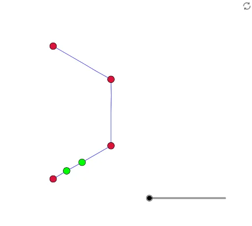
This example demonstrates the generation process of Fractal Curve 4. It involves fractal geometry and power functions. Using the PolyLine and Rotate commands, a series of rotated points are constructed to form a complex fractal pattern. Suitable for high school and above students to learn fractal geometry and function transformations.
GeoGebra Commands & Parameters
PolyLine(A, E, F, B) → fRotate(A1, (4 * π / 3), B) → B1Rotate(Translate[A1, D - B], (2 * π / 3), D) → C1Rotate(Dilate[{A1, B1, C1}, 0.5], (-2 * π / 6)) → A2Rotate(A2, (4 * π / 3), B) → B2Rotate(Translate[A2, D - B], (2 * π / 3), D) → C2Rotate(Dilate[{A2, B2, C2}, 0.500000000000002], (-2 * π / 6)) → A3Rotate(A3, (4 * π / 3), B) → B3Rotate(Translate[A3, D - B], (2 * π / 3), D) → C3Rotate(Dilate[{A3, B3, C3}, 0.500000000000004], (-2 * π / 6)) → A4Rotate(A4, (4 * π / 3), B) → B4Rotate(Translate[A4, D - B], (2 * π / 3), D) → C4Rotate(Dilate[{A4, B4, C4}, 0.500000000000006], (-2 * π / 6)) → A5Rotate(A5, (4 * π / 3), B) → B5Rotate(Translate[A5, D - B], (2 * π / 3), D) → C5Rotate(Dilate[{A5, B5, C5}, 0.500000000000008], (-2 * π / 6)) → A6Rotate(A6, (4 * π / 3), B) → B6Rotate(Translate[A6, D - B], (2 * π / 3), D) → C6Rotate(Dilate[{A6, B6, C6}, 0.50000000000001], (-2 * π / 6)) → A7Rotate(A7, (4 * π / 3), B) → B7Rotate(Translate[A7, D - B], (2 * π / 3), D) → C7Rotate(Dilate[{A7, B7, C7}, 0.50000000000001], (-2 * π / 6)) → A8Rotate(A8, (4 * π / 3), B) → B8Rotate(Translate[A8, D - B], (2 * π / 3), D) → C8
AI Drawing Prompt Reference
Draw a fractal curve by repeatedly rotating, translating, and scaling a series of shapes. Start with an initial quadrilateral, then apply rotations and transformations to each shape, scaling it down each time, to create a complex, recursive fractal pattern that demonstrates transformations and power functions.
The prompt above was compiled from the original drawing commands and is for reference only.