
Fourier Series Example 2: Square Wave Approximation and Harmonic Summation
Loading the math board and drawing, please wait…
In collections
UQ-Applied Mathematical Analysis
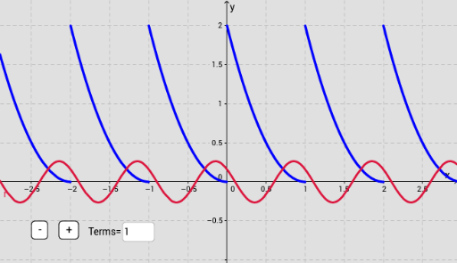
①This example demonstrates how a Fourier series approximates a periodic square wave by summing harmonic sine and cosine terms, with adjustable number of terms to visualize convergence. ②Core mathematical concepts include Fourier series expansion, orthogonality of trigonometric functions, harmonic superposition, partial sums, and the Gibbs phenomenon near discontinuities. ③Construction uses GeoGebra commands such as Sequence to generate coefficient sequences an and bn, Append to build cumulative partial sums, Textfield and InputBox for interactive parameter entry, and buttons to control animation; key objects include functions f, g, n, an, bn, list1, list2, a_0, A0, A1, B1, and input boxes. ④Suitable for university-level calculus, signal processing, or engineering mathematics courses to explore Fourier approximation and harmonic analysis interactively.
GeoGebra Commands & Parameters
Sequence((2 / p * Integral[(f(x) * cos((((i * x) * 2) * π / p))), (-p), 0]), i, 1, n) → anSequence((2 / p * Integral[(f(x) * sin((((i * x) * 2) * π / p))), (-p), 0]), i, 1, n) → bnSequence((Element[an, i] * cos((((π * i) * 2 / p) * x))) + (Element[bn, i] * sin((((π * i) * 2 / p) * x))), i, 1, n) → list1Sequence((2 / p * Integral[(f(x) * cos((((i * x) * 2) * π / p))), (-p), 0]), i, 2, n) → an'Sequence((2 / p * Integral[(f(x) * sin((((i * x) * 2) * π / p))), (-p), 0]), i, 2, n) → bn'Append(A1, an') → an''Append(B1, bn') → bn''Sequence((Element[an'', i] * cos((((π * i) * 2 / p) * x))) + (Element[bn'', i] * sin((((π * i) * 2 / p) * x))), i, 1, n) → list2Textfield(A0) → InputBox1Textfield(A1) → InputBox2Textfield(B1) → InputBox3Textfield(n) → InputBox4