
Forest Decay
Loading the math board and drawing, please wait…
In collections
Geom. & Alg.: Exponential Functions & Logarithms
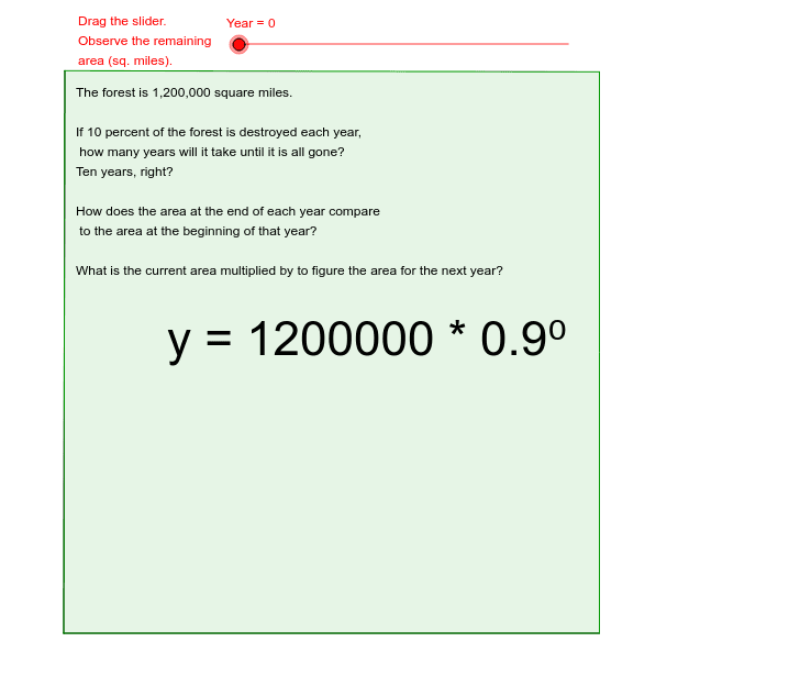
This example visually and numerically demonstrates exponential decay. It involves key mathematical concepts such as exponential functions and their decay properties. Using GeoGebra commands like Point, Segment, OrthogonalLine, etc., key objects such as years and decay rates are constructed. Suitable for high school and above students or teachers for teaching or self-study.
GeoGebra Commands & Parameters
Point(Circle[A, 20 * 0.9^(Year)]) → BSegment(A, B) → aPoint(Circle[A, 20 * 0.9^(Year)]) → CSegment(A, C) → bOrthogonalLine(B, a) → cOrthogonalLine(C, b) → dIntersect(d, c) → DPolygon(A, C, D, B) → poly1, a_1, c_1, d_1, b_1Text(SqMiles) → text2
AI Drawing Prompt Reference
Draw a graph showing forest area decay over time. Start with an initial forest area of 20 square miles, decaying annually at a rate of 0.9. Draw line segments from the origin to each point, then draw perpendicular lines to these segments, find their intersection points, and finally enclose a polygon with these points and the origin.
The prompt above was compiled from the original drawing commands and is for reference only.