
Flux and Circulation: Circle & Square
Loading the math board and drawing, please wait…
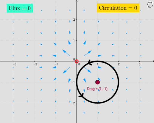
This example demonstrates the concepts of flux and circulation on a circle and a square. Key mathematical concepts include vectors, derivatives, and integrals. Using GeoGebra commands such as CurveCartesian, Circle, Derivative, and Sum, dynamic geometric figures are constructed to illustrate the changes in flux and circulation. Suitable for high school math education and students learning calculus.
GeoGebra Commands & Parameters
CurveCartesian((Radius * cos(((2 * π) * t))) + x(Drag), (Radius * sin(((2 * π) * t))) + y(Drag), t, 0, 1) → path_cSequence(Sequence[Vector[(j, k), (j + (scale * F_1(j, k)), k + (scale * F_2(j, k)))], j, xmin, xmax, xstep], k, ymin, ymax, ystep) → vFieldLine(I, xAxis) → fLine(J, xAxis) → gLine(K, xAxis) → hSequence(Segment[Rotate[curlPt - (0.2, 0), k + curlAngle, curlPt], Rotate[curlPt + (0.2, 0), k + curlAngle, curlPt]], k, 0, 2.0944, 1.0472) → spokesCircle(divPt, 0.2) → divGlowCircleCurveCartesian((t * x(Drag)) + ((1 - t) * x(Drag)), (t * (y(Drag) + Side)) + ((1 - t) * y(Drag)), t, 0, 1) → path_{s1}CurveCartesian((t * (x(Drag) - Side)) + ((1 - t) * x(Drag)), (t * (y(Drag) + Side)) + ((1 - t) * (y(Drag) + Side)), t, 0, 1) → path_{s2}CurveCartesian((t * (x(Drag) - Side)) + ((1 - t) * (x(Drag) - Side)), (t * y(Drag)) + ((1 - t) * (y(Drag) + Side)), t, 0, 1) → path_{s3}CurveCartesian((t * x(Drag)) + ((1 - t) * (x(Drag) - Side)), (t * y(Drag)) + ((1 - t) * y(Drag)), t, 0, 1) → path_{s4}Derivative(path_{s1}) → Dpath_{s1}Derivative(path_{s2}) → Dpath_{s2}Derivative(path_{s3}) → Dpath_{s3}Derivative(path_{s4}) → Dpath_{s4}Sum(Sequence[(((F_1(x(path_{s1}(i + dS / 2)), y(path_{s1}(i + dS / 2))), F_2(x(path_{s1}(i + dS / 2)), y(path_{s1}(i + dS / 2)))) * (y(Dpath_{s1}(i + dS / 2)), (-x(Dpath_{s1}(i + dS / 2))))) * dS), i, 0, 1 - dS, dS]) → Flux_{s1}Sum(Sequence[(((F_1(x(path_{s2}(i + dS / 2)), y(path_{s2}(i + dS / 2))), F_2(x(path_{s2}(i + dS / 2)), y(path_{s2}(i + dS / 2)))) * (y(Dpath_{s2}(i + dS / 2)), (-x(Dpath_{s2}(i + dS / 2))))) * dS), i, 0, 1 - dS, dS]) → Flux_{s2}Sum(Sequence[(((F_1(x(path_{s3}(i + dS / 2)), y(path_{s3}(i + dS / 2))), F_2(x(path_{s3}(i + dS / 2)), y(path_{s3}(i + dS / 2)))) * (y(Dpath_{s3}(i + dS / 2)), (-x(Dpath_{s3}(i + dS / 2))))) * dS), i, 0, 1 - dS, dS]) → Flux_{s3}Sum(Sequence[(((F_1(x(path_{s4}(i + dS / 2)), y(path_{s4}(i + dS / 2))), F_2(x(path_{s4}(i + dS / 2)), y(path_{s4}(i + dS / 2)))) * (y(Dpath_{s4}(i + dS / 2)), (-x(Dpath_{s4}(i + dS / 2))))) * dS), i, 0, 1 - dS, dS]) → Flux_{s4}Sum(list1, (s * 4)) → TTSum(Sequence[((path_{s1}(i + dS) - path_{s1}(i)) * (F_1(x(path_{s1}(i + dS / 2)), y(path_{s1}(i + dS / 2))), F_2(x(path_{s1}(i + dS / 2)), y(path_{s1}(i + dS / 2))))), i, 0, s - dS, dS]) → Circ_1Sum(Sequence[((path_{s2}(i + dS) - path_{s2}(i)) * (F_1(x(path_{s2}(i + dS / 2)), y(path_{s2}(i + dS / 2))), F_2(x(path_{s2}(i + dS / 2)), y(path_{s2}(i + dS / 2))))), i, 0, s - dS, dS]) → Circ_2Sum(Sequence[((path_{s3}(i + dS) - path_{s3}(i)) * (F_1(x(path_{s3}(i + dS / 2)), y(path_{s3}(i + dS / 2))), F_2(x(path_{s3}(i + dS / 2)), y(path_{s3}(i + dS / 2))))), i, 0, s - dS, dS]) → Circ_3Sum(Sequence[((path_{s4}(i + dS) - path_{s4}(i)) * (F_1(x(path_{s4}(i + dS / 2)), y(path_{s4}(i + dS / 2))), F_2(x(path_{s4}(i + dS / 2)), y(path_{s4}(i + dS / 2))))), i, 0, s - dS, dS]) → Circ_4Sum(list2, (4 * s)) → TT_2Segment(path_{s1}(0.5), path_{s1}(0.5 + 0.01)) → arrw01Segment(path_{s2}(0.5), path_{s2}(0.5 + 0.01)) → arrw02Segment(path_{s3}(0.5), path_{s3}(0.5 + 0.01)) → arrw03Segment(path_{s4}(0.5), path_{s4}(0.5 + 0.01)) → arrw04Distance(Drag, (0, 0)) → condPolygon(Drag, M, 4) → poly1, i, j, k, l, N, OSum(Sequence[((path_c(i + dS) - path_c(i)) * (F_1(x(path_c(i + dS / 2)), y(path_c(i + dS / 2))), F_2(x(path_c(i + dS / 2)), y(path_c(i + dS / 2))))), i, 0, s2 - dS, dS]) → CircDerivative(path_c) → Dpath_cSum(Sequence[(((F_1(x(path_c(i + dS / 2)), y(path_c(i + dS / 2))), F_2(x(path_c(i + dS / 2)), y(path_c(i + dS / 2)))) * (y(Dpath_c(i + dS / 2)), (-x(Dpath_c(i + dS / 2))))) * dS), i, 0, s2 - dS, dS]) → FluxSegment(path_c(0.3), path_c(0.3 + 0.01)) → arrow01Segment(path_c(0.6), path_c(0.6 + 0.01)) → arrow02CurveCartesian((Radius * cos(((2 * π) * t))) + x(Drag), (Radius * sin(((2 * π) * t))) + y(Drag), t, 0, s2) → partPath_c
AI Drawing Prompt Reference
Draw a circle centered at the draggable point and a square with sides parallel to the x-axis. Add a vector field on the circle to show the direction and strength of the flow. Calculate and draw circulation and flux on the circle and square boundaries, using arrows to indicate.
The prompt above was compiled from the original drawing commands and is for reference only.