
Finite Growth Model Demonstration
Loading the math board and drawing, please wait…
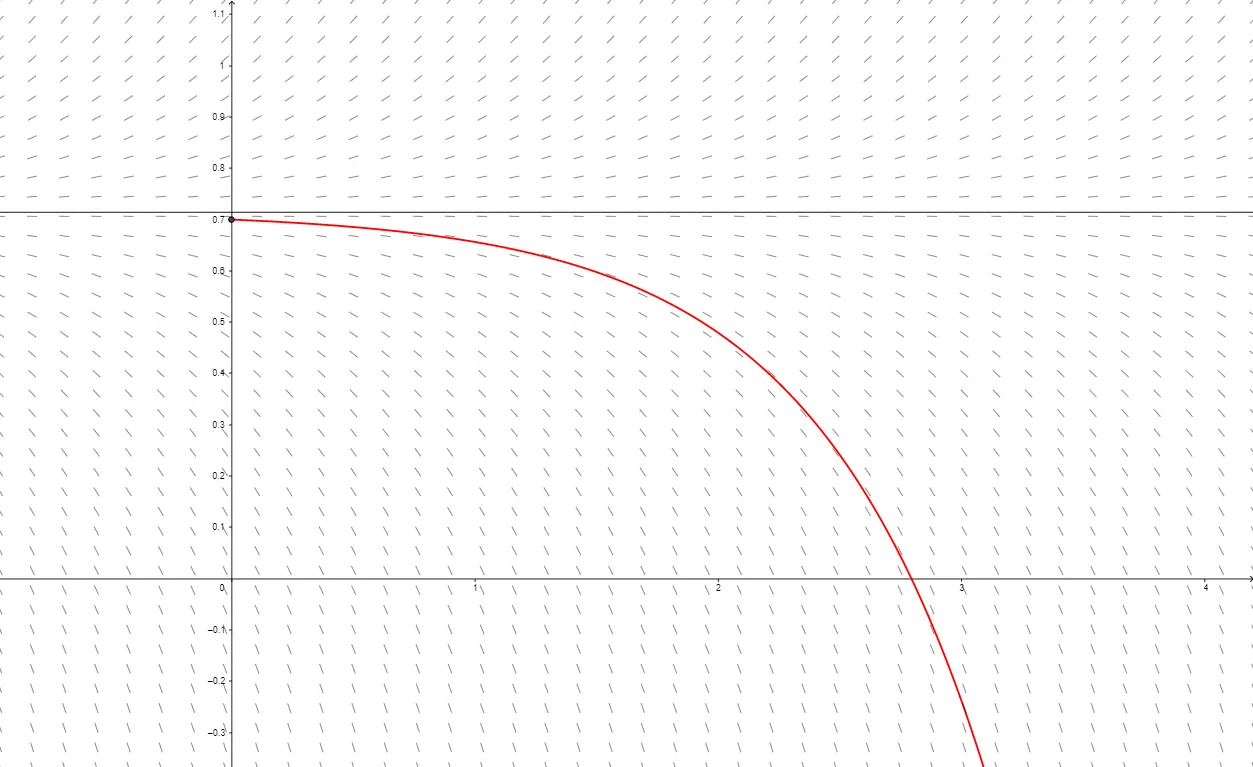
This example demonstrates the finite growth model through graphics, involving core mathematical concepts such as differential equations, continuity, confidence intervals, and integers. Key construction elements include using the SlopeField command to plot the slope field, objects like teind, P0, k, m, A, f, aantal, f′, A1, B1, g, B, i, j, slopefield1, tekst1, h, etc. Suitable for high school and above mathematics learners and researchers.
GeoGebra Commands & Parameters
SlopeField((k * y) - m, 40, 0.5) → slopefield1
AI Drawing Prompt Reference
Create a slope field (direction field) visualization for a finite growth model. Use the differential-equation expression (k*y - m) to define the slope at each point on the plane. Render the field over the specified x–y range with about 40 grid lines and a step size close to 0.5, so the local inclination directions are clearly shown. The goal is to illustrate the qualitative behavior implied by this first-order differential equation, providing an intuitive backdrop for understanding related functions and derivatives.
The prompt above was compiled from the original drawing commands and is for reference only.