
Finding the Area Enclosed by a Polar Curve
Loading the math board and drawing, please wait…
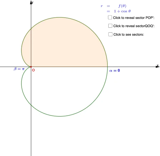
This example demonstrates how to calculate the area enclosed by a polar curve using polar coordinates and integration. It involves constructing a polar curve, computing the area of a circular sector, and applying the integral formula for polar area. The GeoGebra commands include CurveCartesian for curve plotting, CircleSector and Segment for geometric construction, Integral for area calculation, and Midpoint/Rotate for geometric manipulation. Suitable for high school and early university calculus students learning polar coordinate geometry.
GeoGebra Commands & Parameters
CurveCartesian(((1 + cos(t)) * cos(t)), ((1 + cos(t)) * sin(t)), t, (-π), π) → aCurveCartesian(((1 + cos(t)) * cos(t)), ((1 + cos(t)) * sin(t)), t, 0, π) → cFractionText(d) → text1Rotate(Q, α, O) → Q'Angle(Q, O, Q') → βCircleSector(O, Q, Q') → δAFractionText(deltatheta) → text3Segment(O, Q') → fIntersect(f, a) → B, P, F, GRotate(P, (-β), O) → P'Angle(P', O, P) → γCircleSector(O, P', P) → eMidpoint(O, Q) → AMidpoint(O, P) → CMidpoint(P', Q) → DAngle(E, O, Q) → δMidpoint(A, C) → HCircleSector(O, P', P) → gIntegral((1 + cos(x))^(2), theta, theta + deltatheta) → AreaSequence((1 + cos(θ); θ), θ, 0, π, π / n) → l1Ray(O, l1(1)) → mRay(O, l1(2)) → pRay(O, l1(3)) → qRay(O, l1(4)) → rRay(O, l1(5)) → sRay(O, l1(6)) → tRay(O, l1(7)) → f_1Ray(O, l1(8)) → g_1Ray(O, l1(9)) → h_1Ray(O, l1(10)) → i_1Ray(O, l1(11)) → j_1Ray(O, l1(12)) → k_1Ray(O, l1(13)) → l_1Ray(O, l1(14)) → m_1Ray(O, l1(15)) → n_1Ray(O, l1(16)) → p_1Ray(O, l1(17)) → q_1Ray(O, l1(18)) → r_1Ray(O, l1(19)) → s_1Ray(O, l1(20)) → t_1Sequence((1 + cos(θ); θ + π / n), θ, 0, π, π / n) → l2CircleSector(O, l1(1), l2(1)) → Out_1CircleSector(O, l1(2), l2(2)) → Out_2CircleSector(O, l1(3), l2(3)) → Out_3CircleSector(O, l1(4), l2(4)) → Out_4CircleSector(O, l1(5), l2(5)) → Out_5CircleSector(O, l1(6), l2(6)) → Out_6CircleSector(O, l1(7), l2(7)) → Out_7CircleSector(O, l1(8), l2(8)) → Out_8CircleSector(O, l1(9), l2(9)) → Out_9CircleSector(O, l1(10), l2(10)) → Out_{10}CircleSector(O, l1(11), l2(11)) → Out_{11}CircleSector(O, l1(12), l2(12)) → Out_{12}CircleSector(O, l1(13), l2(13)) → Out_{13}CircleSector(O, l1(14), l2(14)) → Out_{14}CircleSector(O, l1(15), l2(15)) → Out_{15}CircleSector(O, l1(16), l2(16)) → Out_{16}CircleSector(O, l1(17), l2(17)) → Out_{17}CircleSector(O, l1(18), l2(18)) → Out_{18}CircleSector(O, l1(19), l2(19)) → Out_{19}CircleSector(O, l1(20), l2(20)) → Out_{20}Sequence((1 + cos(θ + π / n); θ), θ, 0, π, π / n) → l3CircleSector(O, l3(1), l2(1)) → In_1CircleSector(O, l3(2), l2(2)) → In_{2}CircleSector(O, l3(3), l2(3)) → In_4CircleSector(O, l3(4), l2(4)) → In_{3}CircleSector(O, l3(5), l2(5)) → In_5CircleSector(O, l3(6), l2(6)) → In_{6}CircleSector(O, l3(7), l2(7)) → In_7CircleSector(O, l3(8), l2(8)) → In_8CircleSector(O, l3(9), l2(9)) → In_9CircleSector(O, l3(10), l2(10)) → In_{10}CircleSector(O, l3(11), l2(11)) → In_{11}CircleSector(O, l3(12), l2(12)) → In_{12}CircleSector(O, l3(13), l2(13)) → In_{13}CircleSector(O, l3(14), l2(14)) → In_{14}CircleSector(O, l3(15), l2(15)) → In_{15}CircleSector(O, l3(16), l2(16)) → In_{16}CircleSector(O, l3(17), l2(17)) → In_{17}CircleSector(O, l3(18), l2(18)) → In_{18}CircleSector(O, l3(19), l2(19)) → In_{19}CircleSector(O, l3(20), l2(20)) → In_{20}CircleSector(O, l3(1), l2(1)) → Outl_1CircleSector(O, l3(2), l2(2)) → Outl_2CircleSector(O, l3(3), l2(3)) → Outl_1_3CircleSector(O, l3(4), l2(4)) → Outl_4CircleSector(O, l3(5), l2(5)) → Outl_5CircleSector(O, l3(6), l2(6)) → Outl_6CircleSector(O, l3(7), l2(7)) → Outl_7CircleSector(O, l3(8), l2(8)) → Outl_3CircleSector(O, l3(8), l2(8)) → Outl_8CircleSector(O, l3(9), l2(9)) → Outl_9CircleSector(O, l3(10), l2(10)) → Outl_{10}CircleSector(O, l3(11), l2(11)) → Outl_{11}CircleSector(O, l3(12), l2(12)) → Outl_{12}CircleSector(O, l3(13), l2(13)) → Outl_{13}CircleSector(O, l3(14), l2(14)) → Outl_{14}CircleSector(O, l3(15), l2(15)) → Outl_{15}CircleSector(O, l3(16), l2(16)) → Outl_{16}CircleSector(O, l3(17), l2(17)) → Outl_{17}CircleSector(O, l3(18), l2(18)) → Outl_{18}CircleSector(O, l3(19), l2(19)) → Outl_{19}
AI Drawing Prompt Reference
On a coordinate plane, plot a polar-type parametric curve using two parameter ranges: draw one curve for angle parameter from −π to π and another for angle parameter from 0 to π, keeping them as the two reference curves. Select curve points that will act as endpoints of sector constructions, then use rotation about the origin to create a corresponding endpoint related by a measured angle. Construct sector arcs at the origin bounded by the rotated and original endpoints, and include the straight segment(s) connecting the origin to the endpoints. Find intersection points between the constructed sector boundary/segment and the drawn curve(s), then rotate one of the intersection-derived points about the origin by the indicated angle direction to obtain the second endpoint. Add the corresponding sector (arc) around the origin for the rotated configuration, preparing the visual for using the parameter increment as a reference for the area calculation over the interval.
The prompt above was compiled from the original drawing commands and is for reference only.