
Finding Critical Points and Their Nature Using Hessian Matrix
Loading the math board and drawing, please wait…
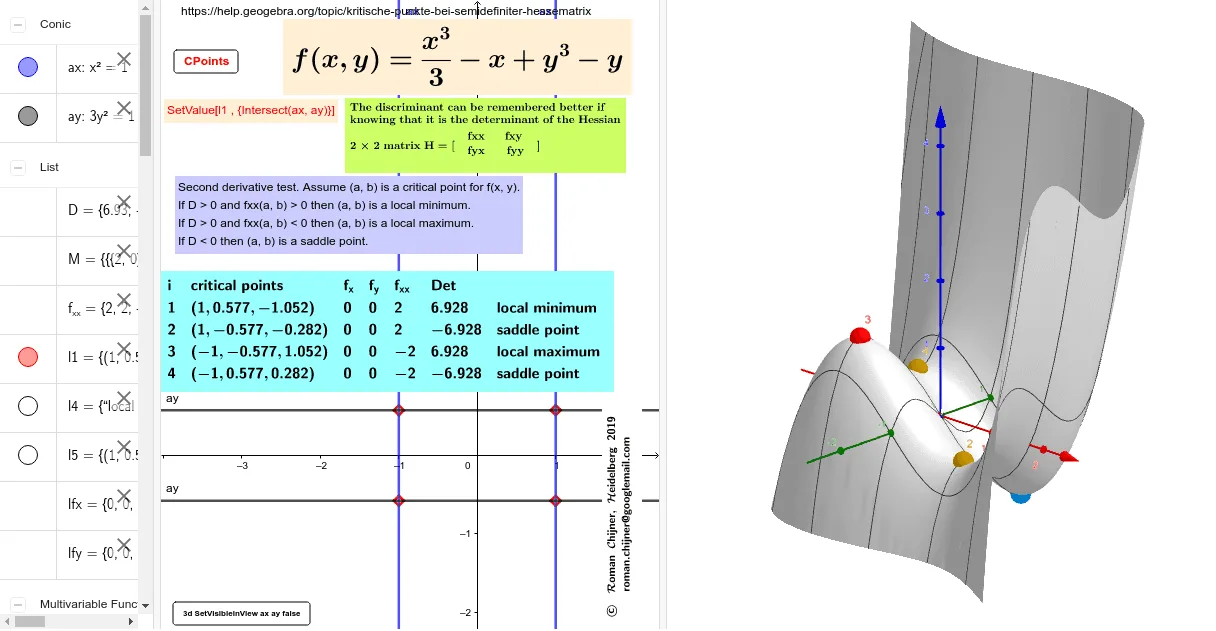
This example demonstrates how to use the Hessian matrix to find the critical points and their nature of a function. Key mathematical concepts include derivatives, Hessian matrix, and function extrema. Using commands like Simplify, Zip, and Sequence, the example constructs the second derivative matrix of the function and determines the nature of the critical points. Suitable for calculus and advanced mathematics courses.
GeoGebra Commands & Parameters
Simplify(Derivative[f, x, 1]) → fxSimplify(Derivative[fx, x, 1]) → fxxSimplify(Derivative[fx, y, 1]) → fxySimplify(Derivative[f, y, 1]) → fySimplify(Derivative[fy, y, 1]) → fyySimplify(Derivative[fy, x, 1]) → fyxZip({{fxx(a), fxy(a)}, {fyx(a), fyy(a)}}, a, l1) → MZip(Determinant[a], a, M) → DZip(fxx(a), a, l1) → f_{xx}Sequence(If[D(i) > 0, If[f_{xx}(i) > 0, "local minimum", "local maximum"], "saddle point"], i, 1, Length[l1]) → l4Zip((x(a), y(a), f(a)), a, l1) → l5Zip(fx(a), a, l1) → lfxZip(fy(a), a, l1) → lfyTableText(Append["i", 1…Length[l1]], Append["critical points", l5], Append["f_{x}", lfx], Append["f_{y}", lfy], Append["f_{xx}", f_{xx}], Append["Det", D], Append["", l4], "v") → text1LaTeX(f, true) → text3RotateText(txt1, 90°) → txt2
AI Drawing Prompt Reference
Plot the function f(x, y) and find its critical points. Use the Hessian matrix to determine the nature of these points, including the second-order partial derivatives matrix, determinant, local minimum, local maximum, and saddle point.
The prompt above was compiled from the original drawing commands and is for reference only.