Filling Curves Interactive Demo

Loading the math board and drawing, please wait…

2019-12-28 16:21

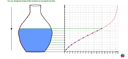
This example demonstrates the generation process and properties of filling curves through interactive means. It involves core mathematical concepts such as function graphs, intersections, symmetry, rational and real numbers. The construction leverages GeoGebra commands/objects like Line, Point, Mirror, Sequence, PolyLine, Sum, Midpoint, Segment, Ellipse, Take, Union, and Vector. It is suitable for high school and above students to understand fractal geometry, parametric equations, and transformation ideas.

GeoGebra Commands & Parameters

Line(B, yAxis) → ff
Point(a) → C1
Point(c_1) → C21
Point(b_1) → C20
Point(a_1) → C19
Point(t) → C18
Point(r) → C17
Point(q) → C16
Point(p) → C15
Point(n) → C14
Point(m) → C13
Point(l) → C12
Point(k) → C11
Point(j) → C10
Point(i) → C9
Point(h_1) → C8
Point(g) → C7
Point(f) → C6
Point(e) → C5
Point(d) → C4
Point(c) → C3
Point(b) → C2
Mirror(C2, ff) → D2
Mirror(C3, ff) → D3
Mirror(C4, ff) → D4
Mirror(C5, ff) → D5
Mirror(C6, ff) → D6
Mirror(C7, ff) → D7
Mirror(C8, ff) → D8
Mirror(C9, ff) → D9
Mirror(C10, ff) → D10
Mirror(C11, ff) → D11
Mirror(C12, ff) → D12
Mirror(C13, ff) → D13
Mirror(C14, ff) → D14
Mirror(C15, ff) → D15
Mirror(C16, ff) → D16
Mirror(C17, ff) → D17
Sequence(abs(x(Object["C" + (t)]) - x(B)), t, 1, 21) → rayon
PolyLine(liste1) → s
Sequence(Element[rayon, k]^(2) + Element[rayon, k + 1]^(2) + (Element[rayon, k] * Element[rayon, k + 1]), k, 1, 20) → volumes
Sum(volumes) → volumenT
Sequence(Sum[First[volumeB, k]], k, 1, 21) → volumeA
Mirror(C18, ff) → D18
Mirror(C19, ff) → D19
Mirror(C20, ff) → D20
Mirror(C21, ff) → D21
Sequence(((20 * Element[volumeA, k]), k), k, 1, 21) → points
Mirror(C1, ff) → D1
PolyLine(liste2) → d_1
Midpoint(C1, D1) → A
Sequence(Segment[Element[points, k], Element[points, k + 1]], k, 1, 19) → liste3
Segment(D1, (10, 0)) → e_1
Sequence(Segment[(k, 0), (k, 20)], k, 0, 20) → traitverti
Sequence(Segment[(0, k), (20, k)], k, 1, 20) → traith
Sequence(Segment[Object["D" + (t)], (0, t - 1)], t, 1, 21) → liste4
Ellipse(D1, C1, C) → f_1
Midpoint(C21, D21) → D
Ellipse(C21, D21, E) → g_1
Sequence(Segment[Element[points, t], (0, t)], t, 1, 21) → liste5
Segment((0, 0), Element[points, 1]) → i_1
Take(liste5, 1, h - 1) → liste7
Take(liste4, 1, h) → liste6
Take(points, 1, h - 1) → haut1
Take(liste1, 1, h) → rec1
Take(liste2, 1, h) → rec2
Union(rec1, rec2) → rec
Sequence(Polygon[Element[liste1, i], Element[liste1, i + 1], Element[liste2, i + 1], Element[liste2, i]], i, 1, Length[liste7]) → liste8
Ellipse(D1, C1, C) → k_1
Ellipse(C21, D21, E) → p_1
Segment(Element[liste1, h], Element[points, h - 1]) → haut
Sequence(G + ((i * AxisStepX[]), 0), i, 0, 20) → liste9
Sequence(G + (0, (i * AxisStepY[])), i, 0, 20) → liste10
Vector(G, H) → u
Vector(G, I) → v
Sequence(Text["" + (i), Element[liste9, i + 1] - (0.2, 0.75)], i, 0, 20) → liste11
Take(volumes, 1, h - 1) → volhaut
Sum(volhaut) → Vol
Take(liste3, 1, h - 2) → liste12

AI Drawing Prompt Reference

Create an interactive filling curve demonstration. Start with a vertical axis of symmetry. Place a sequence of points on one side, connected by a polyline. Reflect each point across the axis to get corresponding points on the other side. Compute horizontal distances from the axis, then use these to build cumulative sums. Map these sums to new points, forming a curve. The figure illustrates symmetry, sequences, and transformations, suitable for exploring fractals and parametric equations.

The prompt above was compiled from the original drawing commands and is for reference only.