
Ferris Wheel Vertical Drop Animation (No Values)
Loading the math board and drawing, please wait…
In collections
Math Year 4 Unit 1
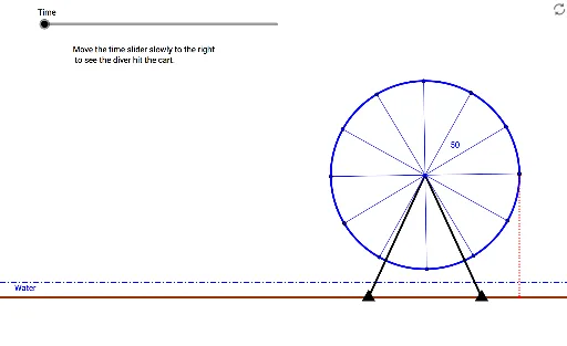
① This GeoGebra example dynamically demonstrates the vertical displacement of a point on a Ferris wheel as it rotates, visually linking circular motion to its vertical projection. ② Core mathematical concepts include trigonometric functions (sine and cosine), parametric equations of a circle, rotation and angle measurement, and vertical distance calculation. ③ Construction uses commands: Circle, Segment, Rotate, Angle, Line, OrthogonalLine, Intersect, and Distance; key objects include Time (slider), Grd (ground), C (center), c (circle), G1/G2 (reference points), a (radius), α (angle), and multiple Zero' points for tracking positions. ④ Suitable for high school students learning trigonometry, circular motion, and geometric transformations, as well as for physics demonstrations of simple harmonic motion.
GeoGebra Commands & Parameters
Circle(C, 50) → cSegment(C, G1) → aSegment(C, G2) → bRotate(Zero, α, C) → Zero'Angle(Zero, C, Zero') → βSegment(C, Zero') → dRotate(Zero, 30° + α, C) → Zero'_1Angle(Zero, C, Zero'_1) → γSegment(C, Zero'_1) → eRotate(Zero, 60° + α, C) → Zero'_2Angle(Zero, C, Zero'_2) → δSegment(C, Zero'_2) → fRotate(Zero, 90° + α, C) → Zero'_3Angle(Zero, C, Zero'_3) → εSegment(Zero'_3, C) → gRotate(Zero, 120° + α, C) → Zero'_4Angle(Zero, C, Zero'_4) → ζSegment(Zero'_4, C) → hRotate(Zero, 150° + α, C) → Zero'_5Angle(Zero, C, Zero'_5) → ηSegment(Zero'_5, C) → iRotate(Zero, 180° + α, C) → Zero'_6Angle(Zero, C, Zero'_6) → θSegment(Zero'_6, C) → jRotate(Zero, 210° + α, C) → Zero'_7Angle(Zero, C, Zero'_7) → ιSegment(Zero'_7, C) → kRotate(Zero, 240° + α, C) → Zero'_8Angle(Zero, C, Zero'_8) → κSegment(Zero'_8, C) → lRotate(Zero, 270° + α, C) → Zero'_9Angle(Zero, C, Zero'_9) → λSegment(Zero'_9, C) → mRotate(Zero, 300° + α, C) → Zero'_{10}Angle(Zero, C, Zero'_{10}) → μSegment(Zero'_{10}, C) → nRotate(Zero, 330° + α, C) → Zero'_{11}Angle(Zero, C, Zero'_{11}) → νSegment(Zero'_{11}, C) → pLine(G1, G2) → qOrthogonalLine(Zero', q) → rIntersect(r, q) → ASegment(Zero', A) → sOrthogonalLine(Zero'_1, d) → tIntersect(d, t) → BOrthogonalLine(Zero'_2, d) → b_1Intersect(b_1, d) → DDistance(D, C) → distanceDCIntersect(f_1, g_1, (12.282854594082735, -17.547711629319735)) → E