
Extreme Distribution of 72 Points on a Sphere: Polyhedron Coloring and Dual Comp
Loading the math board and drawing, please wait…
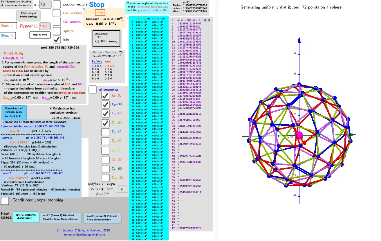
This GeoGebra example demonstrates the extreme distribution of 72 points on the surface of a sphere, constructing the convex hull polyhedron and comparing it with two known but non-extreme configurations having the same number of vertices. The core mathematical concepts include spherical point distribution optimization (such as Thomson or Tammes problems), convex hull construction, polyhedral duality, and visualization of vertices, edges, and faces through coloring. The construction uses GeoGebra commands including Sphere for the base sphere, Text, LaTeX, and TableText for dynamic labels, Zip, If, and Sum for list operations on vertex coordinates and distance calculations, and Append with UnicodeToLetter for data sequencing. Interactive sliders (n, r, i0, j0) and input boxes (InputBox1, InputBox2) allow users to adjust parameters in real time. This resource is suitable for high school to university-level mathematics, particularly for exploring solid geometry, optimization problems, and computational geometry. It serves as an excellent tool for mathematical modeling, competition training, or classroom demonstrations to visualize the relationship between extreme distributions and polyhedral structures.
GeoGebra Commands & Parameters
Text("" + Um1) → txt_pLaTeX(Um1) → lll1_1LaTeX(Um0) → lll0Sphere(O, R) → p1Textfield(n) → InputBox1Textfield(i0) → InputBox2Text(r) → TxtrTextfield(k_1) → InputBox4UnicodeToLetter(34) → u34Textfield(k_2) → InputBox5TableText(ltxt0, ltxt1, "v") → textltxt01Append(A, Sequence[((random(), random(), random()) * R), i, 2, n]) → l2sText(("(up\; to\; 10^{-15})\;\\ accuracy= " * ScientificText[cc, 3]), C, true, true) → text5rZip(Vector[a, a + UnitVector[a]], a, lP') → lVector1Textfield(scale) → InputBox6TableText(Append["i", 1…n], Append[" \fgcolor{orange}{GM :Δφ_i}, rad", l1], Append["\fgcolor{magenta}{GC :Δφ_i} , rad", l1c], "v") → text23Text("\;\;\;\;\;\;\;\;\;\;\;\;\;\fgcolor{" + (If[c', "orange", "brown"]) + "} \boxed{ " + c' + "}\;\;\;\; \;\;\;\;\; \\\;\; ( accuracy- up\; to\;\; 2.*10^{" + k_2 + ("\;})\;\\\;\; ➤➤➤\;\;\;\scalebox{1.3}{ " + (ScientificText[cc, 3])) + "}\;█ ", C, true, true) → text9If(bu, "Animation", "Stop") → bue0Zip(Vector[a, a + (1.5 * UnitVector[b])], a, lP', b, Wi_P) → lVector3Zip(Vector[a, a + (1.5 * UnitVector[b])], a, lP', b, Wi_Pc) → lVector2TableText({Join[{{"n"}, Sequence[i, i, 4, 69 + 3]}], Join[{{" p_n=P_n/[R*n*(n-1)/2]"}, lp}]}, "vl") → txt_lpSum(Flatten[Sequence[Append[Sequence[Element[txt_p, i], i, m1(k), m2(k)], " "], k, 1, 5]]) → txtUm1Zip(Segment[Element[lP', y(a)], Element[lP', z(a)]], a, ll1bb(2)) → ll2Zip(Segment[Element[lP', y(a)], Element[lP', z(a)]], a, ll1bb(3)) → ll3Zip(Segment[Element[lP', y(a)], Element[lP', z(a)]], a, ll1bb(4)) → ll4Zip(Segment[Element[lP', y(a)], Element[lP', z(a)]], a, ll1bb(5)) → ll5Zip(Segment[Element[lP', y(a)], Element[lP', z(a)]], a, ll1bb(6)) → ll6Zip(Segment[Element[lP', y(a)], Element[lP', z(a)]], a, ll1bb(7)) → ll7Zip(Segment[Element[lP', y(a)], Element[lP', z(a)]], a, ll1bb(8)) → ll8Zip(Segment[Element[lP', y(a)], Element[lP', z(a)]], a, ll1bb(9)) → ll9Zip(Segment[Element[lP', y(a)], Element[lP', z(a)]], a, ll1bb(10)) → ll10Zip(Segment[Element[lP', y(a)], Element[lP', z(a)]], a, ll1bb(1)) → ll1
AI Drawing Prompt Reference
Draw a sphere with 72 optimally distributed points, forming a convex polyhedron. Color the vertices, edges, and faces of the polyhedron differently. Adjust parameters n, i0, j0, k1, and k2 to change the number and distribution of points, and observe the changes in the polyhedron.
The prompt above was compiled from the original drawing commands and is for reference only.