
Exponential Growth and Decay
Loading the math board and drawing, please wait…
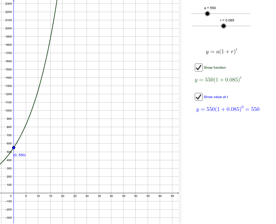
This example demonstrates the graphical phenomena of exponential growth and decay functions. Key mathematical concepts include exponential functions, geometric mean, similar triangles, and rectangle area calculations. Construction involves GeoGebra commands such as Polygon, PointIn, Intersect, DynamicCoordinates, and OrthogonalLine. Suitable for high school mathematics courses or mathematical modeling exercises.
GeoGebra Commands & Parameters
Polygon((0, 0), (0, y(Corner[3])), Corner[3], (x(Corner[3]), 0)) → poly1, d, e, g, hPointIn(poly1) → DIntersect(f, e, (17.78948293511821, 2347.682768423995)) → EDynamicCoordinates(D, If[x(D) < 0, 0, If[x(D) > x(E), x(E), x(D)]], If[x(D) < 0, f(0), If[x(D) > x(E), y(E), f(x(D))]]) → BPointIn(poly1) → AOrthogonalLine(B, xAxis) → i
AI Drawing Prompt Reference
Draw an exponential growth and decay function graph. First, draw a rectangle and place a point D randomly inside it. Then, find the intersection point E of the function f and the rectangle edge e. Adjust the coordinates of point B dynamically based on the position of point D: if D is above the x-axis, B coincides with D; if below, B coincides with the x-axis; if between the x-axis and E, B coincides with E. Finally, draw a vertical line i through point B.
The prompt above was compiled from the original drawing commands and is for reference only.