
Exponential Ball Drop: Dynamic Modeling of Height and Speed
Loading the math board and drawing, please wait…
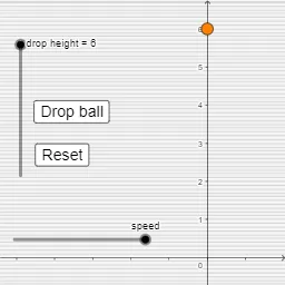
This GeoGebra applet animates a ball dropping from an initial height and demonstrates how the height decreases over time following an exponential decay behavior. The animation is linked to related quantities such as speed and time, letting learners observe how changing parameters affects the motion profile. Key math concepts include exponential functions (decay modeling), logarithms and function relationships, and geometric parameterization using isosceles triangle constraints, together with vector/proportional connections and combinatorial-style parameter bookkeeping. Construction-wise, the model is driven by time, height, the function f, and speed; additional function expressions like h, p, q, r, g1, s, t1, l, m, g, b are used as intermediate parameters to compute the evolving geometry and the graph behavior. Interactive control elements button1–button4 and the running flag going manage the simulation steps, while text1 provides labels for key variables. Suitable for high school through early university classes in function modeling, graphing, and interactive STEM instruction.
GeoGebra Commands & Parameters
Numeric height(6)f(x) = (height * abs((cos(x - 0.1) * ℯ^((-((x - 0.1) / 10))))))Numeric time(0)Numeric speed(20)h(x) = (-16 * x^(2)) + heightp(x) = (-16 * (x(Root[h(x), 2]) - x)^(2)) + (height * ℯ^((-(x / 4))))q(x) = (-16 * (x - x(Root[p, 4]))^(2)) + (height * ℯ^((-(x(Root[p, 4]) / 4))))r(x) = (-16 * (x(Root[q(x), 6]) - x)^(2)) + (height * ℯ^((-(x / 4))))g_{1}(x) = (height * ℯ^(x / -4))y = (-16 * (x - x(Root[r, 8]))^(2)) + (height * ℯ^((-(x(Root[r, 8]) / 4))))t_{1}(x) = (-16 * (x - x(Root[s, 10]))^(2)) + (height * ℯ^((-(x / 4))))y = (-16 * (x - x(Root[t_{1}, 10]))^(2)) + (height * ℯ^((-(x(Root[t_{1}, 10]) / 4))))x(Root[t, 10])x(Root[(-16 * (x - l)^(2)) + (height * ℯ^((-(x / 4)))), 10])y = (-16 * (x - m)^(2)) + (height * ℯ^((-(m / 4))))b(x) = If[0 ≤ x < x(Root[h(x), 2]), (-16 * x^(2)) + height, If[x < x(Root[q(x), 6]), q(x), If[x < x(Root[s(x), 10]), s(x), If[x < x(Root[t(x), 10]), t(x), If[x < x(Root[g(x), 12]), g(x)]]]]](0, b(time))Boolean going(false)
AI Drawing Prompt Reference
Create a coordinate-plane visualization of a dynamic “ball drop” height model with exponential decay. Start by setting an initial height and a time parameter, then define a height function of time that decreases according to an exponential decay term. Include a related speed quantity driven by the same time input. Use a piecewise definition for the height curve so that the active formula switches at boundary times determined by solving for roots (intersection points) in the constructed expressions. Plot the resulting height as a curve versus time, showing the height value at the origin for t=0, and keep an animation-like update flag so learners can observe how changing parameters affects the motion profile and the curve segments.
The prompt above was compiled from the original drawing commands and is for reference only.