Exploring the PDF of Sums of Continuous Random Variables on [0,1]

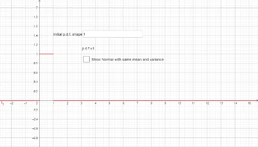
This GeoGebra example demonstrates the probability density function (PDF) of the sum of several continuous random variables (CRVs) each defined on the interval [0,1]. It visually explores how the distribution of the sum evolves as the number of variables increases, illustrating the central limit theorem and the convolution of uniform distributions. The construction uses interactive input via Textfield and InputBox1, numerical integration with the NIntegral command, and the Normal command to generate a normal approximation curve. Multiple function objects (f1 to f12) and line objects (L1 to L12) are used to plot the PDFs for different numbers of summed variables, with sliders (k) and parameters (μ, σ) for adjustment. This resource is suitable for high school or undergraduate probability and statistics courses, helping students understand the transition from uniform to normal distributions and the practical computation of convolutions.