
Euler's Method Differential Equation Solution
Loading the math board and drawing, please wait…
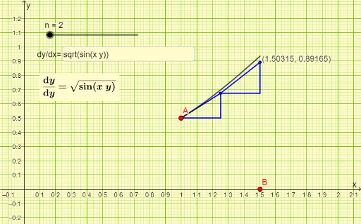
This example demonstrates the step-by-step solution of a differential equation using Euler's method in GeoGebra. It visually illustrates the iterative process of numerical approximation and the application of numerical integration. Key math concepts include differential equations, numerical methods, iterative computation, and function graphing. The construction leverages commands like SolveODE, Point, IterationList, Sequence, NSolveODE, Textfield, and Element, enabling interactive parameter control and result visualization through sliders and input boxes. Ideal for high school students and math enthusiasts studying the principles and implementation of numerical solutions for differential equations.
GeoGebra Commands & Parameters
SolveODE(f, A) → gPoint(xAxis) → BIterationList((x(C) + h, y(C) + (h * f(x(C), y(C)))), C, {A}, n) → l1Sequence((x(Element[l1, v + 1]), y(Element[l1, v])), v, 1, n) → l2Sequence(Segment[Element[l1, v], Element[l1, v + 1]], v, 1, n) → l3Sequence(Segment[Element[l1, v], Element[l2, v]], v, 1, n) → l4Sequence(Segment[Element[l2, v], Element[l1, v + 1]], v, 1, n) → l5NSolveODE({f}, x(A), {y(A)}, x(B)) → numericalIntegral1Textfield(f) → InputBox1Element(l1, n + 1) → C
AI Drawing Prompt Reference
Draw a graph showing Euler's method for solving a differential equation. The graph should include an initial point, a sequence of iterative points, and line segments connecting these points. Users can adjust parameters to observe the numerical approximation process. The graph should clearly show the iterative steps and final result.
The prompt above was compiled from the original drawing commands and is for reference only.