
Euler's Method by Juan Carlos Ponce Campuzano
Loading the math board and drawing, please wait…
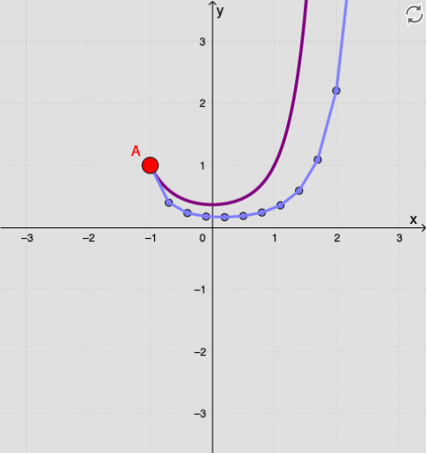
This example demonstrates Euler's method, a numerical technique for solving differential equations. It involves the concept of derivatives in calculus. Using GeoGebra commands like Sequence, SlopeField, and PolyLine, the construction of Euler's method is illustrated. Suitable for high school mathematics education and learning.
GeoGebra Commands & Parameters
Sequence((Element[xns, i], Element[yns, i]), i, 1, 300) → pointsxynsSlopeField(F, Density, scale) → slopefield1PolyLine(pointsxyns) → fSequence(Element[xns, i], i, 1 + n, 11 + n) → list1Sequence(Element[yns, i], i, 1 + n, 11 + n) → list2Sequence(i, i, n, n + 10) → list3Element(list3, D1) → E1Element(list3, D2) → E2Element(list3, D3) → E3Element(list3, D4) → E4Element(list3, D5) → E5Element(list3, D6) → E6Element(list3, D7) → E7Element(list3, D8) → E8Element(list3, D9) → E9Element(list3, D10) → E10Element(list3, D11) → E11Element(list1, D1) → F1Element(list1, D2) → F2Element(list1, D3) → F3Element(list1, D4) → F4Element(list1, D5) → F5Element(list1, D6) → F6Element(list1, D7) → F7Element(list1, D8) → F8Element(list1, D9) → F9Element(list1, D10) → F10Element(list1, D11) → F11Element(list2, D1) → G1Element(list2, D2) → G2Element(list2, D3) → G3Element(list2, D4) → G4Element(list2, D5) → G5Element(list2, D6) → G6Element(list2, D7) → G7Element(list2, D8) → G8Element(list2, D9) → G9Element(list2, D10) → G10Element(list2, D11) → G11TableText({{"n", "x_n", "y_n"}, {E1, F1, G1}, {E2, F2, G2}, {E3, F3, G3}, {E4, F4, G4}, {E5, F5, G5}, {E6, F6, G6}, {E7, F7, G7}, {E8, F8, G8}, {E9, F9, G9}, {E10, F10, G10}, {E11, F11, G11}}, "|_") → text1Textfield(Ax) → InputBox1Textfield(Ay) → InputBox2Textfield(F) → InputBox3Textfield(h) → InputBox4SolveODE(F, x(A), y(A), 100, 0.01) → numericalIntegral1
AI Drawing Prompt Reference
Draw a demonstration of Euler's method, showing a slope field for a differential equation and the numerical solution curve obtained via Euler's method. First, display the slope field, then starting from an initial point, draw points according to the slope of the differential equation and connect these points to form a curve. Finally, list the x and y coordinates for each step in a table on the right side of the graph, along with the initial conditions and step size.
The prompt above was compiled from the original drawing commands and is for reference only.