
Unit Rate Exploration: Secant Line Approximation and Derivative Concept
Loading the math board and drawing, please wait…
In collections
Unit 2 Classwork: Intro to Ratios
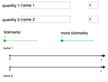
This example demonstrates how to understand the concept of 'how much for one' through secant line approximation. The core mathematical concepts include the geometric meaning of derivatives - secant slope approaching tangent slope, limit thinking, and geometric distribution probability calculation. Using GeoGebra commands like Textfield, InputBox, Point, Segment, Sequence, and GCD, an interactive teaching interface is constructed: by entering different data sets, observe how secant slope approaches tangent slope as the interval shrinks, combined with geometric distribution to verify single event probability. Suitable for middle and high school mathematics courses introducing derivatives, intuitive understanding of limit concepts, and demonstrating geometric distribution in probability and statistics.
GeoGebra Commands & Parameters
Textfield(text4) → InputBox2Textfield(Q1Jump) → InputBox4Textfield(text5) → InputBox3Textfield(Q2Jump) → InputBox5Point(a) → DSegment(A, D) → cSegment(B, C) → dText("20%", (scale - 0.25, y(A) + yOffSet)) → text6Text(8, (scale - 0.12, y(B) + yOffSet)) → text7GCD(Q1Jump, Q2Jump) → gSegment(A, I) → iSegment(B, J) → kText(0, (x(A) - 0.12, y(A) - (1.2 * yOffSet))) → text2Sequence(((e * v), h), v, 0, f) → Q1marksSequence(((e * k), 0), k, 0, f) → Q2marksSequence(Text[(q * Q1Jump), ((e * q) + topxOffSet, y(B) + yOffSet)], q, 1, f) → TextQ1Sequence(Text[(p * Q2Jump), ((e * p) + xOffSet, y(A) + yOffSet)], p, 1, f) → TextQ2Sequence(Text[(q * Q1Jump / 2), ((e / 2 * q) + topxOffSet, y(B) + yOffSet)], q, 1, (f * 2)) → TextQ1split2Sequence(((e / 2 * l), h), l, 0, (f * 2)) → Q1split2Sequence(((e / 2 * k), 0), k, 0, (f * 2)) → Q2split2Sequence(Text[(p * Q2Jump / 2), ((e / 2 * p) + (1.1 * xOffSet), y(A) + yOffSet)], p, 1, (f * 2)) → TextQ2split2Text(0, (x(B) - 0.12, y(B) + (3.2 * yOffSet))) → text3Sequence(((e / s * l), h), l, 0, (f * s)) → Q1splitSequence(((e / s * k), 0), k, 0, (f * s)) → Q2splitSequence(Text[(q * Q1Jump / s), ((e / s * q) + topxOffSet, y(B) + yOffSet)], q, 1, (f * s)) → TextQ1splitSequence(Text[(p * Q2Jump / s), ((e / s * p) + xOffSet, y(A) + yOffSet)], p, 1, (f * s)) → TextQ2split
AI Drawing Prompt Reference
Create a coordinate-plane diagram for the “secant slope approaching tangent slope” idea of derivatives. Use two user-input parameters representing left and right jump counts, and constrain the main interval endpoints via their greatest common divisor. Plot two key point pairs and draw the corresponding line segments to represent two secants over different interval choices. Add on-figure text labels showing a fixed proportion (e.g., 20%) and additional numeric annotations derived from scaled versions of the input parameters, laid out along the same vertical reference lines as the points. Finally, add several sets of labels for progressively smaller interval lengths to visually indicate the shrinking-step (limit) behavior.
The prompt above was compiled from the original drawing commands and is for reference only.