Visualizing Euler's Method for First-Order Differential Equations

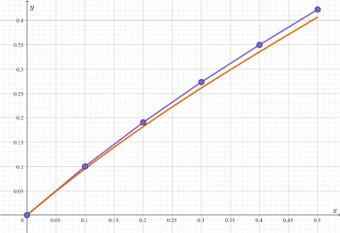
① This GeoGebra example dynamically illustrates Euler's method for numerically solving a first-order ordinary differential equation y'=f(x,y), showing how a polygonal approximation is built step-by-step from an initial condition with a chosen step size. ② Core mathematical concepts include first-order ODEs, numerical integration, Euler's iteration scheme, initial value problems, and the effect of step size on approximation accuracy. ③ Construction highlights: uses IterationList to generate successive points, Sequence for lists, PolyLine to connect points into a broken line, and NSolveODE to compute the exact solution for comparison; interactive Textfield and InputBox elements allow users to input f(x,y), initial values (x₀,y₀), and step size h, with sliders for dynamic parameter adjustment. ④ Suitable for university calculus or differential equations courses, as well as advanced high school mathematics, to help students grasp the fundamentals of numerical methods and error analysis, and to support inquiry-based learning in mathematical experimentation.