
Equiangular Spiral Construction
Loading the math board and drawing, please wait…
In collections
Logarithmic Spiral and Fibonacci Numbers
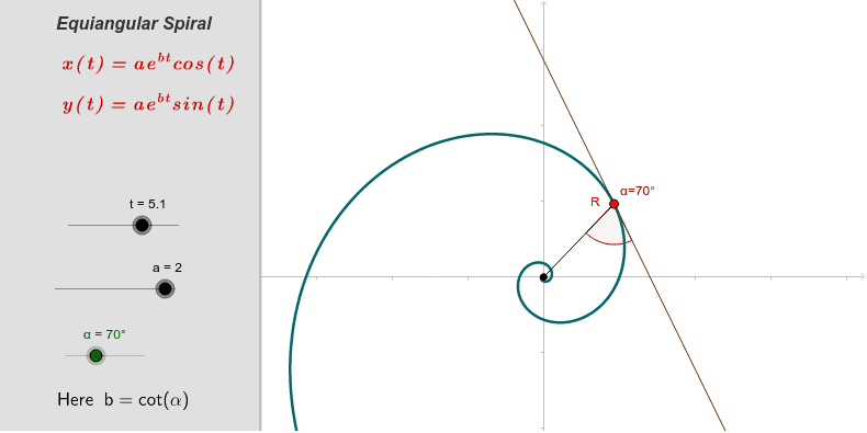
This example demonstrates the construction of an equiangular spiral by dynamically adjusting the constant a and the angle α between the tangent and radius. It involves core mathematical concepts like polar coordinates, trigonometry, and geometric construction. Key GeoGebra commands used include CurveCartesian, Point, Tangent, Segment, Angle, and Polygon. Suitable for high school and above, it illustrates parametric equations, coordinate geometry, and the interactivity of dynamic geometry.
GeoGebra Commands & Parameters
CurveCartesian(((a * ℯ^((b * tt))) * cos(tt)), ((a * ℯ^((b * tt))) * sin(tt)), tt, left, t) → cPoint(c) → RTangent(R, c) → dSegment(O, R) → ePoint(d) → BAngle(O, R, B) → α_1Polygon(Corner[1], (x(Corner[1]) + (0.3 * Distance[Corner[1], Corner[2]]), y(Corner[1])), (x(Corner[4]) + (0.3 * Distance[Corner[1], Corner[2]]), y(Corner[4])), Corner[4]) → poly1, f, g, h, i
AI Drawing Prompt Reference
Draw an equiangular spiral, dynamically adjusting the constant a and the angle α between the tangent and radius to demonstrate core concepts like polar coordinates, trigonometry, and geometric construction. Start by plotting a curve defined by parametric equations, then mark a point on the curve, draw the tangent and radius at that point, measure the angle between them, and finally construct a polygon to illustrate the interactivity of dynamic geometry.
The prompt above was compiled from the original drawing commands and is for reference only.